Sparse Matrices

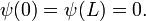
A sparse matrix is a matrix in which most of the entries are zero. Such matrices are very commonly encountered in finite-difference equations. For example, when we discretized the 1D Schrödinger wave equation with Dirichlet boundary conditions, we saw that the Hamiltonian matrix had the tridiagonal form

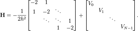
: $\mathbf{H} = -\frac{1}{2h^2} \begin{bmatrix} -2 & 1 \\ 1 & -2 & \ddots \\ & \ddots & \ddots & 1 \\ & & 1 & -2\end{bmatrix} + \begin{bmatrix}V_0 \\ & V_1 \\& & \ddots \\ & & & V_{N-1}\end{bmatrix}.$

Hence, if there are $N$ diagonalization points, the Hamiltonian matrix has a total of $N^2$ entries, but only $O(N)$ of these entries are non-zero.

Sparse matrix algebra

When matrices are sparse, ordinary approaches to matrix arithmetic are wasteful, since a lot of time is spent adding/subtracting or multiplying by zero. For instance, consider the tridiagonal matrix discussed above. To perform the matrix-vector product $\mathbf{H} \vec{\psi}$ in the usual way, for each row $i$ we must compute

$\left(\mathbf{H}\vec{\psi}\right)_i = \sum_{j=0}^{N-1} H_{ij} \psi_j$

: $= \cdots + \left(0\cdot \psi_{i-2}\right) + \left(H_{i,i-1} \cdot \psi_{i-1}\right) + \left(H_{ii} \cdot \psi_{i}\right) + \left(H_{i,i+1} \cdot \psi_{i+1}\right) + \left(0 \cdot \psi_{i+2}\right) + \cdots$

The sum involves $O(N)$ arithmetic operations, so the overall runtime for all $N$ rows is $O(N^2)$ . Clearly, however, most of this time is spent multiplying zero elements of $\mathbf{H}$ with elements of $\vec{\psi}$ , which doesn't contribute to the final result. If we could omit these terms from each sum, the overall runtime for the product would be only $O(N)$ .

However, such savings cannot be achieved with the array data structures we have been using so far. To calculate the matrix-vector product efficiently, the processor needs to know which elements on each row of $\mathbf{H}$ are non-zero, so that it can skip the rest. However, arrays do not provide a fast way to identify which elements are non-zero; the only way to find out is to search the storage blocks one by one, which takes $O(N)$ time on each row. That would wipe out the runtime savings.

Scipy provides special data structures for storing sparse matrices. Unlike ordinary arrays, these data structures are designed so that zero elements are omitted, which not only saves memory, but also allows certain matrix operations to be greatly sped up. Unlike arrays, which can represent not just matrices (2D arrays) but also vectors (1D arrays) and higher-rank tensors (arrays with dimension higher than 2), these sparse data structures are specifically restricted to matrices.

But here's an important catch: there is no single sparse matrix data structure that is ideal for every scenario. Instead, there are multiple sparse matrix formats, and each format is only effective for a certain subset of matrix operations, or for certain kinds of sparse matrices. Therefore, we need to know how the different sparse matrix formats are implemented, as well as their benefits and limitations. Of the many sparse matrix formats offered by Scipy, we will discuss four: List of Lists (LIL), Diagonal Storage (DIA), Compressed Sparse Row (CSR), and Compressed Sparse Column (CSC).

Sparse matrix formats

List of Lists (LIL)

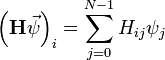
The List of Lists sparse matrix format (which is, for some unknown reason, abbreviated as LIL rather than LOL) is one of the simplest sparse matrix formats. It is shown schematically in the figure below. Each non-zero matrix row is represented by an element in a kind of list structure called a "linked list". Each element in the linked list records the row number, and the column data for the matrix entries in that row. The column data consists of a list, where each list element corresponds to a non-zero matrix element, and stores information about (i) the column number, and (ii) the value of the matrix element.

Fig. 1: A sparse matrix and its representation in List-of-Lists (LIL) format.

Evidently, this format is pretty memory-efficient. The list of rows only needs to be as long as the number of non-zero matrix rows; the rest are omitted. Likewise, each list of column data only needs to be as long as the number of non-zero elements on that row. The total amount of memory required is proportional to the number of non-zero elements, regardless of the size of the matrix itself.

Compared to the other sparse matrix formats which we'll discuss, accessing an individual matrix element in LIL format is relatively slow. This is because looking up a given matrix index $(i,j)$ requires stepping through the row list to find an element with row index $i$ ; and if one is found, stepping through the column row to find index $j$ . Thus, for example, looking up an element in a diagonal $N\times N$ matrix in the LIL format takes $O(N)$ time! As we'll see, the CSR and CSC formats are much more efficient at element access. For the same reason, matrix arithmetic in the LIL format is very inefficient.

One advantage of the LIL format, however, is that it is relatively easy to alter the "sparsity structure" of the matrix. To add a new non-zero element, one simply has to step through the row list, and either (i) insert a new element into the linked list if the row was not previously on the list (this insertion takes $O(1)$ time), or (ii) modify the column list (which is usually very short if the matrix is very sparse).

For this reason, the LIL format is preferred if you need to construct a sparse matrix where the non-zero elements are not distributed in any useful pattern. One way is to create an empty matrix, then fill in the elements one by one, as shown in the following example. The LIL matrix is created by the lil_matrix function, which is provided by the scipy.sparse module.

Here is an example program which constructs a LIL matrix, and prints it:

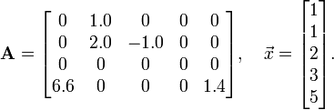
from scipy import *
import scipy.sparse as sp

A = sp.lil_matrix((4,5))     # Create empty 4x5 LIL matrix
A[0,1] = 1.0
A[1,1] = 2.0
A[1,2] = -1.0
A[3,0] = 6.6
A[3,4] = 1.4

## Verify the matrix contents by printing it
print(A)

When we run the above program, it displays the non-zero elements of the sparse matrix:

 (0, 1)	1.0
 (1, 1)	2.0
 (1, 2)	-1.0
 (3, 0)	6.6
 (3, 4)	1.4

You can also convert the sparse matrix into a conventional 2D array, using the toarray method. Suppose we replace the line print(A) in the above program with

B = A.toarray()
print(B)

The result is:

[[ 0.   1.   0.   0.   0. ]
 [ 0.   2.  -1.   0.   0. ]
 [ 0.   0.   0.   0.   0. ]
 [ 6.6  0.   0.   0.   1.4]]

Note: be careful when calling toarray in actual code. If the matrix is huge, the 2D array will eat up unreasonable amounts of memory. It is not uncommon to work with sparse matrices with sizes on the order of $10^5 \times 10^5$ , which can take up less an 1MB of memory in a sparse format, but around 80 GB of memory in array format!

Diagonal Storage (DIA)

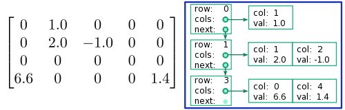
The Diagonal Storage (DIA) format stores the contents of a sparse matrix along its diagonals. It makes use of a 2D array, which we denote by data, and a 1D integer array, which we denote by offsets. A typical example is shown in the following figure:

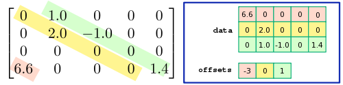
Fig. 2: A sparse matrix and its representation in Diagonal Storage (DIA) format.

Each row of the data array stores one of the diagonals of the matrix, and offsets[i] records which diagonal that row of the data corresponds to, with "offset 0" corresponding to the main diagonal. For instance, in the above example, row 0 of data contains the entries [6.6,0,0,0,0]), and offsets[0] contains the value -3, indicating that the entry 6.6 occurs along the -3 subdiagonal, in column 0. (The extra elements in that row of data lie outside the bounds of the matrix, and are ignored.) Diagonals containing only zero are omitted.

For sparse matrices with very few non-zero diagonals, such as diagonal or tridiagonal matrices, the DIA format allows for very quick arithmetic operations. Its main limitation is that looking up each matrix element requires performing a blind search through the offsets array. That's fine if there are very few non-zero diagonals, as offsets will be small. But if the number of non-zero diagonals becomes large, performance becomes very poor. In the worst-case scenario of an anti-diagonal matrix, element lookup takes $O(N)$ time!

You can create a sparse matrix in the DIA format, using the dia_matrix function, which is provided by the scipy.sparse module. Here is an example program:

from scipy import *
import scipy.sparse as sp

N = 6  # Matrix size
 
diag0 = -2 * ones(N)
diag1 = ones(N)

A = sp.dia_matrix(([diag1, diag0, diag1], [-1,0,1]), shape=(N,N))

## Verify the matrix contents by printing it
print(A.toarray())

Here, the first input to dia_matrix is a tuple of the form (data, offsets), where data and offsets are arrays of the sort described above. This returns a sparse matrix in the DIA format, with the specified contents (the elements in data which lie outside the bounds of the matrix are ignored). In this example, the matrix is tridiagonal with -2 along the main diagonal and 1 along the +1 and -1 diagonals. Running the above program prints the following:

[[-2.  1.  0.  0.  0.  0.]
 [ 1. -2.  1.  0.  0.  0.]
 [ 0.  1. -2.  1.  0.  0.]
 [ 0.  0.  1. -2.  1.  0.]
 [ 0.  0.  0.  1. -2.  1.]
 [ 0.  0.  0.  0.  1. -2.]]

Another way to create a DIA matrix is to first create a matrix in another format (e.g. a conventional 2D array), and provide that as the input to dia_matrix. This returns a sparse matrix with the same contents, in DIA format.

Compressed Sparse Row (CSR)

The Compressed Sparse Row (CSR) format represents a sparse matrix using three arrays, which we denote by data, indices, and indptr. An example is shown in the following figure:

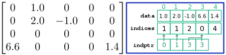
Fig. 3: A sparse matrix and its representation in Compressed Sparse Row (CSR) format.

The array denoted data stores the values of the non-zero elements of the matrix, in sequential order from left to right along each row, then from the top row to the bottom. The array denoted indices records the column index for each of these elements. In the above example, data[3] stores a value of 6.6, and indices[3] has a value of 0, indicating that a matrix element with value 6.6 occurs in column 0. These two arrays have the same length, equal to the number of non-zero elements in the sparse matrix.

The array denoted indptr (which stands for "index pointer") provides an association between the row indices and the matrix elements, but in an indirect manner. Its length is equal to the number of matrix rows (including zero rows). For each row $i$ , if the row is non-zero, indptr[i] records the index in the data and indices arrays corresponding to the first non-zero element on row $i$ . (For a zero row, indptr records the index of the next non-zero element occurring in the matrix.)

For example, consider looking up index $(1,2)$ in the above figure. The row index is 1, so we examine indptr[1] (whose value is 1) and indptr[2] (whose value is 3). This means that the non-zero elements for matrix row 1 correspond to indices $1 \le n < 3$ of the data and indices arrays. We search indices[1] and indices[2], looking for a column index of 2. This is found in indices[2], so we look in data[2] for the value of the matrix element, which is -1.0.

It is clear that looking up an individual matrix element is very efficient. Unlike the LIL format, where we need to step through a linked list, in the CSR format the indptr array lets us to jump straight to the data for the relevant row. For the same reason, the CSR format is efficient for row slicing operations (e.g., A[4,:]), and for matrix-vector products like $\mathbf{A}\vec{x}$ (which involves taking the product of each matrix row with the vector $\vec{x}$ ).

The CSR format does have several downsides. Column slicing (e.g. A[:,4]) is inefficient, since it requires searching through all elements of the indices array for the relevant column index. Changes to the sparsity structure (e.g., inserting new elements) are also very inefficient, since all three arrays need to be re-arranged.

To create a sparse matrix in the CSR format, we use the csr_matrix function, which is provided by the scipy.sparse module. Here is an example program:

from scipy import *
import scipy.sparse as sp

data = [1.0, 2.0, -1.0, 6.6, 1.4]
rows = [0, 1, 1, 3, 3]
cols = [1, 1, 2, 0, 4]

A = sp.csr_matrix((data, [rows, cols]), shape=(4,5))
print(A)

Here, the first input to csr_matrix is a tuple of the form (data, idx), where data is a 1D array specifying the non-zero matrix elements, idx[0,:] specifies the row indices, and idx[1,:] specifies the column indices. Running the program produces the expected results:

 (0, 1)	1.0
 (1, 1)	2.0
 (1, 2)	-1.0
 (3, 0)	6.6
 (3, 4)	1.4

The csr_matrix function figures out and generates the three CSR arrays automatically; you don't need to work them out yourself. But if you like, you can inspect the contents of the CSR arrays directly:

>>> A.data
array([ 1. ,  2. , -1. ,  6.6,  1.4])
>>> A.indices
array([1, 1, 2, 0, 4], dtype=int32)
>>> A.indptr
array([0, 1, 3, 3, 5], dtype=int32)

(There is an extra trailing element of 5 in the indptr array. For simplicity, we didn't mention this in the above discussion, but you should be able to figure out why it's there.)

Another way to create a CSR matrix is to first create a matrix in another format (e.g. a conventional 2D array, or a sparse matrix in LIL format), and provide that as the input to csr_matrix. This returns the specified matrix in CSR format. For example:

>>> A = sp.lil_matrix((6,6))
>>> A[0,1] = 4.0
>>> A[2,0] = 5.0
>>> B = sp.csr_matrix(A)

Compressed Sparse Column (CSC)

The Compressed Sparse Column (CSC) format is very similar to the CSR format, except that the role of rows and columns is swapped. The data array stores non-zero matrix elements in sequential order from top to bottom along each column, then from the left-most column to the right-most. The indices array stores row indices, and each element of the indptr array corresponds to one column of the matrix. An example is shown below:

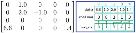
Fig. 4: A sparse matrix and its representation in Compressed Sparse Column (CSC) format.

The CSC format is efficient at matrix lookup, column slicing operations (e.g., A[:,4]), and vector-matrix products like $\vec{x}^{\,T} \mathbf{A}$ (which involves taking the product of the vector $\vec{x}$ with each matrix column). However, it is inefficient for row slicing (e.g. A[4,:]), and for changes to the sparsity structure.

To create a sparse matrix in the CSC format, we use the csc_matrix function. This is analogous to the csr_matrix function for CSR matrices. For example,

>>> from scipy import *
>>> import scipy.sparse as sp
>>> data = [1.0, 2.0, -1.0, 6.6, 1.4]
>>> rows = [0, 1, 1, 3, 3]
>>> cols = [1, 1, 2, 0, 4]
>>> 
>>> A = sp.csc_matrix((data, [rows, cols]), shape=(4,5))
>>> A
<4x5 sparse matrix of type '<class 'numpy.float64'>'
  with 5 stored elements in Compressed Sparse Column format>

Using sparse matrices

Sparse matrix formats should be used, instead of conventional 2D arrays, when dealing sparse matrices of size $10^3\times 10^3$ or larger. (For matrices of size $100\times 100$ or less, the differences in performance and memory usage are usually negligible.)

Usually, it is good to choose either the CSR or CSC format, depending on what mathematical operations you intend to perform. You can construct the matrix either (i) directly, by means of a (data, idx) tuple as described above, or (ii) by creating an LIL matrix, filling in the desired elements, and then converting it to CSR or CSC format.

If you are dealing with a sparse matrix that is "strongly diagonal" (i.e., the non-zero elements occupy a very small number of diagonals, such as a tridiagonal matrix), then you can consider using the DIA format. The main advantage of the DIA format is that it is very easy to construct, by supplying a (data, offsets) input to the dia_matrix function, as described above. However, the format usually does not perform significantly better than CSR/CSC; and if the matrix is not strongly diagonal, its performance is much worse.

Another common way to construct a sparse matrix is to use the scipy.sparse.diags or scipy.sparse.spdiags functions. These functions let you specify the contents of the matrix in terms of its diagonals, as well as which sparse format to use. The two functions have slightly different calling conventions; see the documentation for details.

The `dot` method

Each sparse matrix has a dot method, which calculates the product of the matrix with an input (in the form of a 1D or 2D array, or sparse matrix), and returns the result. For sparse matrix products, this method should be used instead of the stand-alone function, similarly named dot, which is used for non-sparse matrix products. The sparse matrix method makes use of matrix sparsity to speed up the calculation of the product. Typically, the CSR format is faster at this than the other sparse formats.

For example, suppose we want to calculate the product $\mathbf{A} \vec{x}$ , where

: $\mathbf{A} = \begin{bmatrix}0 & 1.0 & 0 & 0 & 0 \\ 0 & 2.0 & -1.0 & 0 & 0 \\ 0 & 0 & 0 & 0 & 0 \\ 6.6 & 0 & 0 & 0 & 1.4\end{bmatrix}, \quad \vec{x} = \begin{bmatrix}1\\1\\2\\3 \\5\end{bmatrix}.$

This could be accomplished with the following program:

from scipy import *
import scipy.sparse as sp

data = [1.0, 2.0, -1.0, 6.6, 1.4]
rows = [0, 1, 1, 3, 3]
cols = [1, 1, 2, 0, 4]
A = sp.csr_matrix((data, [rows, cols]), shape=(4,5))
x = array([1.,1.,2.,3.,5.])

y = A.dot(x)

print(y)

Running this program gives the expected result:

[  1.    0.    0.   13.6]

`spsolve`

The spsolve function, provided in the scipy.sparse.linalg module, is a solver for a sparse linear system of equations. It takes two inputs, $\mathbf{A}$ and $\mathbf{b}$ , where $\mathbf{A}$ should be a sparse matrix; $\mathbf{b}$ can be either sparse, or an ordinary 1D or 2D array. It returns the $\mathbf{x}$ which solves the linear equations $\mathbf{x}$ . The return value can be either a conventional array or a sparse matrix, depending on whether $\mathbf{b}$ is sparse.

For sparse problems, you should always use spsolve instead of scipy.linalg.solve (the usual solver for non-sparse problems). Here is an example program showing spsolve in action:

from scipy import *
import scipy.sparse as sp
import scipy.sparse.linalg as spl

## Make a sparse matrix A and a vector x
data = [1.0, 1.0, 1.0, 1.0, 1.0]
rows = [0, 1, 1, 3, 2]
cols = [1, 1, 2, 0, 3]
A = sp.csr_matrix((data, [rows, cols]), shape=(4,4))
b = array([1.0, 5.0, 3.0, 4.0])

## Solve Ax = b
x = spl.spsolve(A, b)
print(" x = ", x)

## Verify the solution:
print("Ax = ", A.dot(x))
print(" b = ", b)

Running the program gives:

 x =  [ 4.  1.  4.  3.]
Ax =  [ 1.  5.  3.  4.]
 b =  [ 1.  5.  3.  4.]

`eigs`

For eigenvalue problems involving sparse matrices, one typically does not attempt to find all the eigenvalues (and eigenvectors). Sparse matrices are often so huge that solving the full eigenvalue problem would take an impractically long time, even if we receive a speedup from sparse matrix arithmetic. Luckily, in most situations we only need to find a subset of the eigenvalues (and eigenvectors). For example, after discretizing the 1D Schrödinger wave equation, we are normally only interested in the several lowest energy eigenvalues.

The eigs function, provided in the scipy.sparse.linalg module, is an eigensolver for sparse matrices. Unlike the eigensolvers we have previously discussed, such as scipy.linalg.eig, the eigs function only returns a specified subset of the eigenvalues and eigenvectors.

The eigsh function is similar to eigs, except that it is specialized for Hermitian matrices. Both functions make use of a low-level numerical eigensolver library named ARPACK, which is also used by GNU Octave, Matlab, and many other numerical tools. We will not discuss how the algorithm works.

The first input to eigs or eigsh is the matrix for which we want to find the eigenvalues. Several other optional inputs are also accepted. Here are the most commonly-used ones:

The optional parameter named k specifies the number of eigenvalues to find (the default is 6).
The optional parameter named M, if supplied, specifies a right-hand matrix for a generalized eigenvalue problem.
The optional parameter named sigma, if supplied, should be a number; it means to find the k eigenvalues which are closest to that number.
The optional parameter named which specifies which eigenvalues to find, using a criteria different from sigma: 'LM' means to find the eigenvalues with the largest magnitudes, 'SM' means to find those with the smallest magnitudes, etc. You cannot simultaneously specify both sigma and which. When finding small eigenvalues, it is usually better to use sigma instead of which (see the discussion in the next section).
The optional parameter named return_eigenvectors, if True (the default), means to return both eigenvalues and eigenvectors. If False, the function returns the eigenvalues only.

For the full list of inputs, see the full function documentation for eigs and eigsh.

By default, eigs and eigsh return two values: a 1D array (which is complex for eigs and real for eigsh) containing the found eigenvalues, and a 2D array where each column is one of the corresponding eigenvectors. If the optional parameter named return_eigenvectors is set to False, then only the 1D array of eigenvalues is returned.

In the next section, we will see an example of using eigsh.

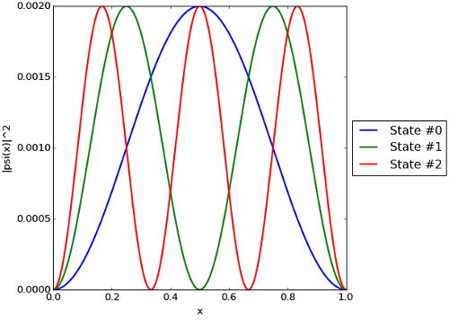
Example: particle-in-a-box problem

To demonstrate the use of sparse matrices for solving finite-difference equations, we consider the 1D particle-in-a-box problem. This consists of the 1D time-independent Schrödinger wave equation,

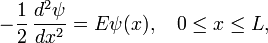
: $-\frac{1}{2} \, \frac{d^2\psi}{dx^2} = E\psi(x), \quad 0 \le x \le L,$

together with the Dirichlet boundary conditions

: $\psi(0) = \psi(L) = 0.$

The analytic solution is well known to us; up to a normalization factor, the eigenstates and energy eigenvalues are

: $\psi_m(x) = \sin\Big(m\pi x / L\Big),\quad E_m = \frac{1}{2}\, \left(\frac{m\pi}{L}\right)^2, \quad m = 1, 2, 3, \dots$

We will write a program that seeks a numerical solution. Using the three-point rule to discretize the second derivative, the finite-difference matrix equations become

: $-\frac{1}{2h^2}\begin{bmatrix} -2 & 1 \\ 1 & -2 & \ddots \\ & \ddots & \ddots & 1 \\ & & 1 & -2\end{bmatrix} \begin{bmatrix}\psi_0 \\ \psi_1 \\ \vdots \\ \psi_{N-1}\end{bmatrix} = E \begin{bmatrix}\psi_0 \\ \psi_1 \\ \vdots \\ \psi_{N-1}\end{bmatrix},$

where

: $h = \frac{L}{N + 1}, \quad \psi_n = \psi\Big(x = h(n+1)\Big)$

The following program constructs the finite-difference matrix equation, and displays the first three solutions:

from scipy import *
import scipy.sparse as sp
import scipy.sparse.linalg as spl
import matplotlib.pyplot as plt

## Solve the 1D particle-in-a-box problem for box length L,
## using N discretization points.  The parameter nev is the
## number of eigenvalues/eigenvectors to find.  Return three
## arrays E, psi, and x.  E stores the energy eigenvalues;
## psi stores the (non-normalized) eigenstates; and x stores
## the discretization points.
def particle_in_a_box(L, N, nev=3):
    dx = L/(N+1.0)
    x  = linspace(dx, L-dx, N)
    I  = ones(N)
    ## Set up the finite-difference matrix.
    H  = sp.dia_matrix(([I, -2*I, I], [-1,0,1]), shape=(N,N))
    H *= -0.5/(dx*dx)
    ## Find the lowest eigenvalues and eigenvectors.
    E, psi = spl.eigsh(H, k=nev, sigma=-1.0)
    return E, psi, x

def particle_in_a_box_demo():
    E, psi, x = particle_in_a_box(1.0, 1000)

    ## Print the energy eigenvalues.
    print(E)

    ## Plot |psi(x)|^2 vs x for each solution found.
    fig = plt.figure()
    axs = plt.subplot(1,1,1)
    for n in range(len(E)):
        fig_label = "State #" + str(n)
        plt.plot(x, abs(psi[:,n])**2, label=fig_label, linewidth=2)
    plt.xlabel('x')
    plt.ylabel('|psi(x)|^2')

    ## Shrink the axis by 20%, so the legend can fit.
    box = axs.get_position()
    axs.set_position([box.x0, box.y0, box.width * 0.8, box.height])
    ## Print the legend.
    plt.legend(loc='center left', bbox_to_anchor=(1, 0.5))
    plt.show()

particle_in_a_box_demo()

The Hamiltonian matrix, which is tridiagonal, is constructed in the DIA sparse matrix format. The eigenvalues and eigenvectors are found with eigsh, which can be used because the Hamiltonian matrix is known to be Hermitian. Notice that we call eigsh using the sigma parameter, telling the eigensolver to find the eigenvalues closest in value to -1.0:

    E, psi = spl.eigsh(H, k=nev, sigma=-1.0)

This will find the lowest energy eigenvalues because, in this case, all energy eigenvalues are positive. (We use -1.0 instead of 0.0, because the algorithm does not work well when sigma is exactly zero.) If there is a negative potential present, we would have to find a different estimate for the lower bound of the energy eigenvalues, and pass that to sigma.

Alternatively, we could have called eigsh with an input which='SA'. This would tell the eigensolver to find the eigenvalue with the smallest value. We avoid doing this because the ARPACK eigensolver algorithm is relatively inefficient at finding small eigenvalues in which mode (and it can sometimes even fail to converge, if k is too small). Typically, if you are able to deduce a lower bound for the desired eigenvalues, it is preferable to use sigma.

Running the program prints the lowest energy eigenvalues:

[  4.93479815  19.73914399  44.41289171]

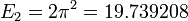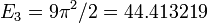This agrees well with the analytical results $E_1 = \pi^2/2 = 4.934802$ , $E_2 = 2\pi^2 = 19.739208$ , and $E_3=9\pi^2/2 = 44.413219$ . It also produces the plot shown below, which is likewise as expected.