Scipy Tutorial (part 2)

This is part 2 of the Scientific Python tutorial.

Sequential data structures

In the previous part of the tutorial, we worked through a simple example of a Scipy program which calculates the electric potential produced by a collection of charges in 1D. At the time, we did not explain much about the data structures that we were using to store numerical information (such as the values of the electric potential at various points). Let's do that now.

There are three common data structures that will be used in a Scipy program for scientific computing: arrays, lists, and tuples. These structures store linear sequences of Python objects, similar to the concept of "vectors" in physics and mathematics. However, these three types of data structures all have slightly different properties, which you should be aware of.

Arrays

An array is a data structure that contains a sequence of numbers. Let's do a quick recap. From a fresh Python command prompt, type the following:

>>> from scipy import *
>>> x = linspace(-0.5, 0.5, 9)
>>> x
array([-0.5  , -0.375, -0.25 , -0.125,  0.   ,  0.125,  0.25 ,  0.375,  0.5  ])

The first line, as usual, is used to import the scipy module. The second line creates an array named x by calling linspace, which is a function defined by scipy. With the given inputs, the function returns an array of 9 numbers between -0.5 and 0.5, inclusive. The third line shows the resulting value of x.

The array data structure is provided specifically by the Scipy scientific computing module. Arrays can only contain numbers (furthermore, each individual array can only contain numbers of one type, e.g. integers or complex numbers; we'll discuss this in the next article). Arrays also support special facilities for doing numerical linear algebra. They are commonly created using one of these functions from the scipy module:

linspace, which creates an array of evenly-spaced values between two endpoints.
arange, which creates an array of integers in a specified range.
zeros, which creates an array whose elements are all 0.0.
ones, which creates an array whose elements are all 1.0.
empty, which creates an array whose elements are uninitialized (this is usually used when you want to set the elements later).

Of these, we've previously seen examples of the linspace and zeros functions being used. As another example, to create an array of 500 elements all containing the number -1.2, you can use the ones function and a multiplication operation:

x = -1.2 * ones(500)

An alternative method, which is slightly faster, is to generate the array using empty and then use the fill method to populate it:

x = empty(500); x.fill(-1.2)

One of the most important things to know about an array is that its size is fixed at the moment of its creation. When creating an array, you need to specify exactly how many numbers you want to store. If you ever need to revise this size, you must create a new array, and transfer the contents over from the old array. (For very big arrays, this might be a slow operation, because it involves copying a lot of numbers between different parts of the computer memory.)

You can pass arrays as inputs to functions in the usual way (e.g., by supplying its name as the argument to a function call). We have already encountered the len function, which takes an array input and returns the array's length (an integer). We have also encountered the abs function, which accepts an array input and returns a new array containing the corresponding absolute values. Similar to abs, many mathematical functions and operations accept arrays as inputs; usually, this has the effect of applying the function or operation to each element of the input array, and returning the result as another array. The returned array has the same size as the input array. For example, the sin function with an array input x returns another array whose elements are the sines of the elements of x:

>>> y = sin(x)
>>> y
array([-0.47942554, -0.36627253, -0.24740396, -0.12467473,  0.        ,
        0.12467473,  0.24740396,  0.36627253,  0.47942554])

You can access individual elements of an array with the notation a[j], where a is the variable name and j is an integer index (where the first element has index 0, the second element has index 1, etc.). For example, the following code sets the first element of the y array to the value of its second element:

>>> y[0] = y[1]
>>> y
array([-0.36627253, -0.36627253, -0.24740396, -0.12467473,  0.        ,
        0.12467473,  0.24740396,  0.36627253,  0.47942554])

Negative indices count backward from the end of the array. For example:

>>> y[-1]
0.47942553860420301

Instead of setting or retrieving individual values of an array, you can also set or retrieve a sequence of values. This is referred to as slicing, and is described in detail in the Scipy documentation. The basic idea can be demonstrated with a few examples:

>>> x[0:3] = 2.0
>>> x
array([ 2.   ,  2.   ,  2.   , -0.125,  0.   ,  0.125,  0.25 ,  0.375,  0.5  ])

The above code accesses the elements in array x, starting from index 0 up to but not including 3 (i.e. indices 0, 1, and 2), and assigns them the value of 2.0. This changes the contents of the array x.

>>> z = x[0:5:2]
>>> z
array([ 2.,  2.,  0.])

The above code retrieves a subset of the elements in array x, starting from index 0 up to but not including 5, and stepping by 2 (i.e., the indices 0, 2, and 4), and then groups those elements into an array named z. Thereafter, z can be treated as an array.

Finally, arrays can also be multidimensional. If we think of an ordinary (1D) array as a vector, then a 2D array is equivalent to a matrix, and higher-dimensional arrays are like tensors. We will see practical examples of higher-dimensional arrays later. For now, here is a simple example:

>>> y = zeros((4,2))     # Create a 2D array of size 4x2
>>> y[2,0] = 1.0
>>> y[0,1] = 2.0
>>> y
array([[ 0.,  2.],
       [ 0.,  0.],
       [ 1.,  0.],
       [ 0.,  0.]])

Lists

There is another type of data structure called a list. Unlike arrays, lists are built into the Python programming language itself, and are not specific to the Scipy module. Lists are general-purpose data structures which are not optimized for scientific computing (for example, we will need to use arrays, not lists, when we want to do linear algebra).

The most convenient thing about Python lists is that you can specify them explicitly, using [...] notation. For example, the following code creates a list named u, containing the integers 1, 1, 2, 3, and 5:

>>> u = [1, 1, 2, 3, 5]
>>> u
[1, 1, 2, 3, 5]

This way of creating lists is also useful for creating Scipy arrays. The array function accepts a list as an input, and returns an array containing the same elements as the input list. For example, to create an array containing the numbers 0.2, 0.1, and 0.0:

>>> x = array([0.2, 0.1, 0.0])
>>> x
array([ 0.2,  0.1,  0. ])

In the first line, the square brackets create a list object containing the numbers 0.2, 0.1, and 0.0, then passes that list directly as the input to the array function. The above code is therefore equivalent to the following:

>>> inputlist = [0.2, 0.1, 0.0]
>>> inputlist
[0.2, 0.1, 0.0]
>>> x = array(inputlist)
>>> x
array([ 0.2,  0.1,  0. ])

Usually, we will do number crunching using arrays rather than lists. However, sometimes it is useful to work directly with lists. One convenient thing about lists is that they can contain arbitrary Python objects, of any data type; by contrast, arrays are allowed only to contain numerical data.

For example, a Python list can store character strings:

>>> u = [1, 2, 'abracadabra', 3]
>>> u
[1, 2, 'abracadabra', 3]

And you can set or retrieve individual elements of a Python list in the same way as an array:

>>> u[1] = 0
>>> u
[1, 0, 'abracadabra', 3]

Another great advantage of lists is that, unlike arrays, you can dynamically increase or decrease the size of a list:

>>> u.append(99)                    # Add 99 to the end of the list u
>>> u.insert(0, -99)                # Insert -99 at the front (index 0) of the list u
>>> u
[-99, 1, 0, 'abracadabra', 3, 99]
>>> z = u.pop(3)                    # Remove element 3 from list u, and name it z
>>> u
[-99, 1, 0, 3, 99]
>>> z
'abracadabra'

Aside: about methods

In the above example, append, insert, and pop are called methods. You can think of a method as a special kind of function which is "attached" to an object and relies upon it in some way. Just like a function, a method can accept inputs, and give a return value. For example, when u is a list, the code

z = u.pop(3)

means to take the list u, find element index 3 (specified by the input to the method), remove it from the list, and return the removed list element. In this case, the returned element is named z. See here for a summary of Python list methods. We'll see more examples of methods as we go along.

Tuples

Apart from lists, Python provides another kind of data structure called a tuple. Whereas lists can be constructed using square bracket [...] notation, tuples can be constructed using parenthetical (...) notation:

>>> v = (1, 2, 'abracadabra', 3)
>>> v
(1, 2, 'abracadabra', 3)

Like lists, tuples can contain any kind of data type. But whereas the size of a list can be changed (using methods like append, insert, and pop, as described in the previous subsection), the size of a tuple is fixed once it's created, just like an array.

Tuples are mainly used as a convenient way to "group" or "ungroup" named variables. Suppose we want to split the contents of v into four separate named variables. We could do it like this:

>>> dog, cat, apple, banana = v
>>> dog
1
>>> cat
2
>>> apple 
'abracadabra'
>>> banana
3

On the left-hand side of the = sign, we're actually specifying a tuple of four variables, named dog, cat, apple, and banana. In cases like this, it is OK to omit the parentheses; when Python sees a group of variable names separated by commas, it automatically treats that group as a tuple. Thus, the above line is equivalent to

>>> (dog, cat, apple, banana) = v

We saw a similar example in the previous part of the tutorial, where there was a line of code like this:

pmin, pmax = -50, 50

This assigns the value -50 to the variable named pmin, and 50 to the variable named pmax. We'll see more examples of tuple usage as we go along.

Improving the program

Let's return to the program for calculating the electric potential, which we discussed in the previous part of the tutorial, and improve it further. These improvements will show off some more advanced features of Python and Scipy which are good to know about.

We'll also make one substantive change in the physics: instead of treating the particles as point-like objects, we'll assume that they have a finite radius $R$ , with all the charge concentrated at the surface. Hence, the potential produced by a particle of total charge $q_0$ and position $x_0$ will have the form

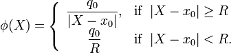
: $\phi(X) = \left\{\begin{array}{cl} \displaystyle \frac{q_0}{|X-x_0|},&\mathrm{if}\;\;|X-x_0| \ge R \\\displaystyle \frac{q_0}{R} &\mathrm{if}\;\;|X-x_0| < R. \end{array}\right.$

Open a few Python file, and call it potentials2.py. Write the following into it:

from scipy import *
import matplotlib.pyplot as plt

## Return the potential at measurement points X, due to particles
## at positions xc and charges qc.  xc, qc, and X must be 1D arrays,
## with xc and qc of equal length.  The return value is an array
## of the same length as X, containing the potentials at each X point.
def potential(xc, qc, X, radius=5e-2):
    assert xc.ndim == qc.ndim == X.ndim == 1
    assert len(xc) == len(qc)
    assert radius > 0.

    phi = zeros(len(X))
    for j in range(len(xc)):
        dphi = qc[j] / abs(X - xc[j])
        dphi[abs(X - xc[j]) < radius] = qc[j] / radius
        phi += dphi
    return phi

## Plot the potential produced by N particles of charge 1, distributed
## randomly between x=-1 and x=1.
def potential_demo(N=20):
    X = linspace(-2.0, 2.0, 200)
    qc = ones(N)

    from scipy.stats import uniform 
    xc = uniform(loc=-1.0, scale=2.0).rvs(size=N)

    phi = potential(xc, qc, X)

    fig_label = 'Potential from ' + str(N) + ' particles'
    plt.plot(X, phi, 'ro', label=fig_label)
    plt.ylim(0, 1.25 * max(phi))
    plt.legend()
    plt.xlabel('r')
    plt.ylabel('phi')
    plt.show()

potential_demo(100)

We will now go through the changes that we've made in the program.

Optional function parameters

As before, we define a function named potential, whose job is to compute the electric potential produced by a collection of particles in 1D. However, you might notice a change in the function header:

def potential(xc, qc, X, radius=5e-2):

We have added an optional parameter, specified as radius=5e-2. An optional parameter is a parameter which has a default value. In this case, the optional parameter is named radius, and its default value is 5e-2 (which means $5\times10^{-2}$ ; you can also write it as 0.05, which is equivalent). If you call the function omitting the last input, the value will be assumed to be 0.05. If you supply an explicit value for the last input, that overrides the default.

If a function call omits a non-optional parameter (which as xc), that is a fatal error: Python will stop the program with an error message.

Assert statements

In the function body, we have added the following three lines:

    assert xc.ndim == qc.ndim == X.ndim == 1
    assert len(xc) == len(qc)
    assert radius > 0.

The assert statement is a special Python statement which checks for the truth value of the following expression; if that expression is false, the program will stop and an informative error message will be displayed.

Here, we use the assert statements to check that

xc, qc, and X are all 1D arrays (note: the == Python operator checks for numerical equality)
xc has the same length as qc
radius has a positive value (note: 0. is Python short-hand for the number 0.0).

Similar to writing comments, adding assert statements to your program is good programming practice. They are used to verify that the assumptions made by the rest of the code (e.g., that the xc and qc arrays have equal length) are indeed met. This ensures that if we make a programming mistake (e.g., supplying arrays of incompatible size as inputs), the problem will surface as soon as possible, rather than letting the program continue to run and causing a more subtle error later on.

Advanced slicing

Inside the for loop, we have changed the way the potential is computed:

    for j in range(len(xc)):
        dphi = qc[j] / abs(X - xc[j])
        dphi[abs(X - xc[j]) < radius] = qc[j] / radius
        phi += dphi

As discussed above, we are now considering particles of finite size rather than point particles, so the potential is constant at distances below the particle radius. This is accomplished using an advanced array slicing technique.

For each particle $j$ , the potential is computed in three steps:

Calculate the potential using the regular formula $q_j / |X-x_j|$ , and save those values into an array, one for each value of $X$ .
Find the indices of that array which correspond to values with $|X - x_j| < R$ , and overwrite those elements with the constant value $q_j/R$ . To find the relevant indices, we make use of the following slicing feature: if a comparison expression is supplied as an index, that refers to those indices for which the comparison is true. In this case, the comparison expression is abs(X-xc[j]) < radius, which refers to the indices of $X$ which are below the minimum radius. These indices are the ones in the dphi array that we want to overwrite.
Add the result to the total potential.

Demo function

Finally, we have a "demo" or ("demonstration") function to make the appropriate plots:

## Plot the potential produced by N particles of charge 1, distributed
## randomly between x=-1 and x=1.
def potential_demo(N=20):
    X = linspace(-2.0, 2.0, 200)
    qc = ones(N)

    from scipy.stats import uniform 
    xc = uniform(loc=-1.0, scale=2.0).rvs(size=N)

    phi = potential(xc, qc, X)

    fig_label = 'Potential from ' + str(N) + ' particles'
    plt.plot(X, phi, 'ro', label=fig_label)
    plt.ylim(0, 1.25 * max(phi))
    plt.legend()
    plt.xlabel('r')
    plt.ylabel('phi')
    plt.show()

potential_demo(100)

Whereas our previous program put the plotting stuff at "top level", here we encapsulate the plotting code in a potential_demo() function. This function is called by the top-level statement potential_demo(100), which occurs at the very end of the program.

It is useful to do this because if, in the future, you want the program demonstrate something else (e.g. producing a different kind of plot), it won't be necessary to delete the potential_demo function (and risk having to rewrite it if you change your mind). Instead, you can write another demo function, and revise that single top-level statement to call the new demo function instead.

The potential_demo function provides another example of using optional parameters. It accepts a parameter N=20, specifying the number of particles to place. When the program runs, however, the function is invoked through the top-level statement potential_demo(100), i.e. with an actual input of 100 which overrides the default value of 20. If the top-level statement had instead been potential_demo(), then the default value of 20 would be used.

Sampling random variables

The demo function generates N particles with random positions. This is done using this code:

    from scipy.stats import uniform 
    xc = uniform(loc=-1.0, scale=2.0).rvs(size=N)

The first line imports a function named uniform from the scipy.stats module, which is a module that implements random number distributions. As this example shows, import statements don't have to be top-level statements. In some cases, we might choose to perform an import only when a particular function runs (usually, this is done if that function is the only one in the program relying on that module).

The uniform function returns an object which corresponds to a particular uniform distribution. One of the methods of this object, named rvs, generates an array of random numbers drawn from that distribution.

Plotting

After computing the total potential using a call to the potential function, we plot it:

   fig_label = 'Potential from ' + str(N) + ' particles'
   plt.plot(X, phi, 'ro', label=fig_label)

To begin with, concentrate on the second line. This is a slightly more sophisticated use of Matplotlib's plot function than what we had the last time.

The first two arguments, as before, are the x and y coordinates for the plot. The next argument, 'ro', specifies that we want to plot using red circles, rather than using lines with the default color.

The fourth argument, label=fig_label, specifies some text with which to label the plotted curve. It is often useful to associate each curve in a figure with a label (though, in this case, the figure contains only one curve).

This way of specifying a function input, which has the form FOO=BAR, is something we have not previously seen. It relies on a feature known as keyword arguments. In this case, label is the keyword (the name of the parameter we're specifying), and fig_label is the value (which is a string object; we'll discuss this below). Keyword arguments allow the caller of a function to specify optional parameters in any order. For example,

   plt.plot(X, phi, 'ro', label=fig_label, linewidth=2)

is equivalent to

   plt.plot(X, phi, 'ro', linewidth=2, label=fig_label)

The full list of keywords for the plot function is given is its documentation.

Constructing a label string

Next, we turn to the line

   fig_label = 'Potential from ' + str(N) + ' particles'

which creates a Python object named fig_label, which is used for labeling the curve. This kind of object is called a character string (or just string for short).

On the right-hand side of the above statement, we build the contents of the string from several pieces. This is done in order to get a different string for each value of N. The + operator "concatenates" strings, joining the strings to its left and right into a longer string. In this case, the string fig_label consists of the following shofter strings, concatenated together:

A string containing the text 'Potential from '.
A string containing the numerical value of N, in text form. This is computed using the str function, which converts numbers into their corresponding string representations.
A string containing the text ' particles'.

The rest of the potential_demo function is relatively self-explanatory. The ylim function specifies the lower and upper limits of the plot's y-axis (there is a similar xlim function, which we didn't use). The plt.legend() statement causes the curve label to be shown in a legend included in the plot. Finally, the xlabel and ylabel functions add string labels to the x and y axes.

Running the program

Now save your potential2.py program, and run it. (Reminder: you can do this by typing python -i potential2.py from the command line on GNU/Linux, or F5 in the Windows GUI, or import potential2 from the Python command line). The resulting figure looks like this:

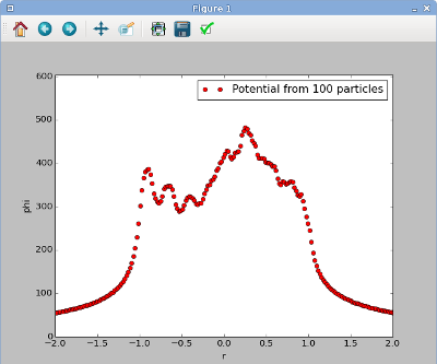
Computational physics notes | Prev: Scipy tutorial Next: Numbers, arrays, and scaling