Numerical Linear Algebra
Much of scientific programming involves handling numerical linear algebra. This is because a huge number of numerical problems which occur in science can be reduced to linear algebra problems. It is very important to know how to formulate these linear algebra problems, and how to solve them numerically.
Contents[hide] |
Array representations of vectors, matrices, and tensors
Thus far, we have discussed simple "one-dimensional" (1D) arrays, which are linear sequences of numbers. In linear algebra terms, 1D arrays represent vectors. The array length corresponds to the "vector dimension" (e.g., a 1D array of length 3 corresponds to a 3-vector). In accordance with Scipy terminology, we will use the work "dimension" to refer to the dimensionality of the array (called the rank in linear algebra), and not the vector dimension.
You are probably familiar with the fact that vectors can be represented using index notation, which is pretty similar to Python's notation for addressing 1D arrays. Consider a length- vector
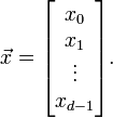
The  th element can be written as
![x_j \quad \leftrightarrow\quad \texttt{x[j]},](PH4505_files/64e075760ccb5708c6e5ad59654de9b1.png)
where 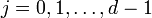 .
The notation on the left is mathematical index notation, and the
notation on the right is Python's array notation. Note that we are
using 0-based indexing, so that the first element has index 0 and the
last element has index
.
The notation on the left is mathematical index notation, and the
notation on the right is Python's array notation. Note that we are
using 0-based indexing, so that the first element has index 0 and the
last element has index  .
.
A matrix is a collection of numbers organized using two
indices, rather than a single index like a vector. Under 0-based
indexing, the elements of an  matrix are:
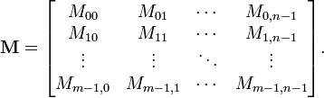
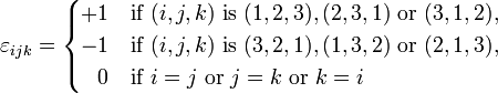
More generally, numbers that are organized using multiple indices are collectively referred to as tensors. Tensors can have more than two indices. For example, vector cross products are computed using the Levi-Civita tensor  , which has three indices:
Multi-dimensional arrays
In Python, tensors are represented by multi-dimensional arrays,
which are similar to 1D arrays except that they are addressed using
more than one index. For example, matrices are represented by 2D
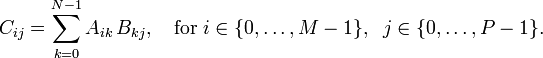
arrays, and the  th component of an matrix is written in Python notation as follows:
![M_{ij} \quad \leftrightarrow\quad \texttt{M[i,j]} \quad\quad \mathrm{for} \;\;i=0,\dots,m-1, \;\;j=0,\dots,n-1.](PH4505_files/477d8a6c631abfdc759768daf37d5432.png)
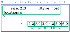
The way multi-dimensional arrays are laid out in memory is very similar to the memory layout of 1D arrays. There is a book-keeping block, which is associated with the array name, and which stores information about the array size (including the number of indices and the size of each index), as well as the memory location of the array contents. The elements lie in a sequence of storage blocks, in a specific order (depending on the array size). This arrangement is shown schematically in Fig. 1.
When Python needs to access any element of of a multi-dimensional
array, it knows exactly which memory location the element is stored in.
The location can be worked out from the size of the multi-dimensional
array, and the memory location of the first element. In Fig. 1, for
example, M is a  array, containing 6 storage blocks laid out in a specific sequence. If we need to access
 M[1,1], Python knows that it needs to jump to the storage block four blocks down from the  block. Hence, reading/writing the elements of a multi-dimensional aray is an
  operation, just like for 1D arrays.
In the following subsections, we will describe how multi-dimensional arrays can be created and manipulated in Python code.
Note: There is also a special Scipy class called matrix which can be used to represent matrices. Don't use this.
It's a layer on top of Scipy's multi-dimensional array facilities,
mostly intended as a crutch for programmers transitioning from Matlab.
Arrays are better to use, and more consistent with the rest of Scipy.
|
Creating multi-dimensional arrays
You can create a 2D array with specific elements using the array command, with an input consisting of a list of lists:
>>> x = array([[1., 2., 3.], [4., 5., 6.]])
>>> x
array([[ 1.,  2.,  3.],
       [ 4.,  5.,  6.]])
The above code creates a 2D array (i.e. a matrix) named x. It is a array, containing the elements  ,
,  ,
,  , etc. Similarly, you can create a 3D array by supplying an input consisting of a list of lists of lists; and so forth.
It is more common, however, to create multi-dimensional arrays using ones or zeros.
These functions return arrays whose elements are all initialized to
0.0 and 1.0, respectively. (You can then assign values to the elements
as desired.) To do this, instead of specifying a number as the input
(which would create a 1D array of that size), you should specify a tuple as the input. For example,
>>> x = zeros((2,3))
>>> x
array([[ 0.,  0.,  0.],
       [ 0.,  0.,  0.]])
>>>
>>> y = ones((3,2))
>>> y
array([[ 1.,  1.],
       [ 1.,  1.],
       [ 1.,  1.]])
There are many more ways to create multi-dimensional arrays, which we'll discuss when needed.
Basic array operations
To check on the dimension of an array, consult its ndim slot:
>>> x = zeros((5,4))
>>> x.ndim
2
To determine the exact shape of the array, use the shape slot (the shape is stored in the form of a tuple):
>>> x.shape
(3, 5)
To access the elements of a multi-dimensional array, use square-bracket notation: M[2,3], T[0,4,2], etc. Just remember that each component is zero-indexed.
Multi-dimensional arrays can be sliced, similar to 1D arrays. There is one important feature of multi-dimensional slicing: if you specify a single value as one of the indices, the slice results in an array of smaller dimensionality. For example:
>>> x = array([[1., 2., 3.], [4., 5., 6.]])
>>> x[:,0]
array([ 1.,  4.])
In the above code, x is a 2D array of size . The slice ![x[:,0]](PH4505_files/991131fbca6a3b63e6795f609870bc00.png) specifies the value 0 for index 1, so the result is a 1D array containing the elements
specifies the value 0 for index 1, so the result is a 1D array containing the elements ![[x_{00}, x_{10}]](PH4505_files/21b0db7bafc9a6b6e834493cae310204.png) .
.
If you don't specify all the indices of a multi-dimensional
array, the omitted indices implicitly included, and run over their
entire range. For example, for the above x array,
>>> x[1]
array([ 4.,  5.,  6.])
This is also equivalent to x[1,:].
Arithmetic operations
The basic arithmetic operations can all be performed on multi-dimensional arrays, and act on the arrays element-by-element. For example,
>>> x = ones((2,3))
>>> y = ones((2,3))
>>> z = x + y
>>> z
array([[ 2.,  2.,  2.],
       [ 2.,  2.,  2.]])
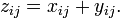
You can think of this in terms of index notation:
What is the runtime for performing such arithmetic operations on
multi-dimensional arrays? With a bit of thinking, we can convince
ourselves that the runtime scales linearly with the number of elements
in the multi-dimensional array, because the arithmetic operation is
performed on each individual index. For example, the runtime for adding
a pair of  matrices scales as
  .
.
Important note: The multiplication operator * also acts element-by-element. It does not refer to matrix multiplication! For example,
>>> x = ones((2,3))
>>> y = ones((2,3))
>>> z = x * y
>>> z
array([[ 1.,  1.,  1.],
       [ 1.,  1.,  1.]])
In index notation, we can think of the * operator as doing this:

By contrast, matrix multiplication is 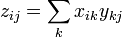 . We'll see how this is accomplished in the next subsection.
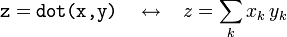
The dot operation
The most commonly-used function for array multiplication is the dot function, which takes two array inputs x and y and returns their "dot product". It constructs a product by summing over the last index of array x, and over the next-to-last index of array y (or over its last index, if y
is a 1D array). This may sound like a complicated rule, but you should
be able to convince yourself that it corresponds to the appropriate
type of multiplication operation for the most common cases encountered
in linear algebra:
- If
xandyare both 1D arrays (vectors), thendotcorresponds to the usual dot product between two vectors:
- If
xis a 2D array andyis a 1D array, thendotcorresponds to right-multiplying a matrix by a vector:
- If
xis a 1D array andyis a 2D array, thendotcorresponds to left-multiplication:
- If
xandyare both 2D arrays,dotcorresponds to matrix multiplication:
- The rule applies to higher-dimensional arrays as well. For example, two rank-3 tensors are multiplied together in this way:
Should you need to perform more general products than what the dot function provides, you can use the tensordot function. This takes two array inputs, x and y, and a tuple of two integers specifying which components of x and y to sum over. For example, if x and y are 2D arrays,

What is the runtime for dot and tensordot? Consider a simple case: matrix multiplication of an matrix with an  matrix. In index notation, this has the form
The resulting matrix has a total of  indices to be computed. Each of these calculations requires a sum involving
  arithmetic operations. Hence, the total runtime scales as
  .
By similar reasoning, we can figure out the runtime scaling for any
tensor product between two tensors: it is the product of the sizes of
the unsummed indices, times the size of the summed index. For example,
for a
.
By similar reasoning, we can figure out the runtime scaling for any
tensor product between two tensors: it is the product of the sizes of
the unsummed indices, times the size of the summed index. For example,
for a tensordot product between an  tensor and a
  tensor, summing over the last index of each tensor, the runtime would scale as
 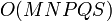 .
.
Linear equations
In physics, we are often called upon to solve linear equations of the form

where  is some
  matrix, and both
  and
and  are vectors for length
  . Given and , the goal is to solve for .
It's an important and useful skill to recognize linear systems of equations when they arise in physics problems. Such equations can arise in many diverse contexts; we will give a couple of simple examples below.
| Example | Suppose there is a set of electrically charged point particles at positions  . We do not know the value of the electric charges, but we able to measure the electric potential at any point . We do not know the value of the electric charges, but we able to measure the electric potential at any point  . The electric potential is given by . The electric potential is given by
|
| |
If we measure the potential at positions,  , how can the charges , how can the charges  be deduced? be deduced?
| |
To do this, let us write the equation for the electric potential at point  as: as:
| |
![\phi(\vec{r}_i) = \sum_{j=0}^{N-1} \left[\frac{1}{|\vec{r}_i-\vec{R}_j|}\right] \, q_j.](PH4505_files/3c323ae32459293dd01b78125c6e52b8.png)
| |
This has the form  , where , where  , ,  , and the unknowns are , and the unknowns are  . .
|
| Example | Linear systems of equations commonly appear in circuit theory. For example, consider the following parallel circuit of power supplies and resistances:
|

| |
Assume the voltage on the right-hand side of the circuit is  . Given the resistances . Given the resistances  and the EMFs and the EMFs  , how do we find the left-hand voltage , how do we find the left-hand voltage  and the currents and the currents  ? ?
| |
| We follow the usual laws of circuit theory. Each branch of the parallel circuit obeys Ohm's law, | |
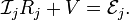
| |
| Furthermore, the currents obey Kirchoff's law (conservation of current), so | |

| |
We can combine these  equations into a matrix equation of the form equations into a matrix equation of the form  : :
| |
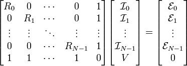
| |
| Here, the unknown vector consists of the currents passing through the branches of the circuit, and the potential .
|
Direct solution
Faced with a system of linear equations, one's first instinct is usually to solve for by inverting the matrix :

Don't do this. It is mathematically correct, but numerically inefficient. As we'll see, computing the matrix inverse  , and then right-multiplying by , involves more steps than simply solving the equation directly
To solve a system of linear equations, use the solve function from the scipy.linalg module. (You will need to import scipy.linalg explicitly, because it is a submodule of scipy and does not get imported by our usual from scipy import * statement.) Here is an example:
>>> A = array([[1., 2., 3.], [2., 4., 0.], [1., 3., 9.]])
>>> b = array([6., 6., 9.])
>>>
>>> import scipy.linalg as lin
>>> x = lin.solve(A, b)
>>> x
array([ 9., -3.,  1.])
We can verify that this is indeed the solution:
>>> dot(A, x)              # This should equal b.
array([ 6.,  6.,  9.])
The direct solver uses an algorithm known as Gaussian elimination, which we'll discuss in the next article. The runtime of Gaussian elimination is  , where is the size of the linear algebra problem.
The reason we avoid solving linear equations by inverting the matrix
is that the matrix inverse is itself calculated using the Gaussian
elimination algorithm! If you are going to use Gaussian elimination
anyway, it is far better to apply the algorithm directly on the desired and  . Solving by calculating involves about twice as many computational steps.
Exercises
- Write Python code to construct a 3D array of size
 corresponding to the Levi-Civita tensor,
Then, using thetensordotfunction, verify the identity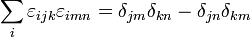 .
.
Computational physics notes | Prev: Numbers, arrays, and scaling Next: Gaussian elimination
