Scipy Tutorial
This is a tutorial for Scientific Python (Scipy), a scientific computing module for the Python programming language. There are a couple of other introductions to Scipy online, which are of excellent quality:
- Scipy Tutorial: the official tutorial.
- More Python Scientific Lecture Notes: a textbook which goes in-depth into using Scipy.
The present tutorial serves a slightly different purpose. It acts as a "walkthrough", guiding you through each step of writing a basic but complete Scipy program. You can use this as the basis for a more complete exploration of Scipy, possibly using the above online resources.
I will assume no pre-existing knowledge of the Python programming language. Programming language constructs are explained as they appear. But if you need more an even more basic tutorial on Python, feel free to consult any of the dozens available online.
Contents[hide] |
Preliminaries
Installing Python and Scipy
If you don't have Scipy installed yet, there are plenty of installation options, detailed here.
- If you are using GNU/Linux, Python is probably already
installed, so just install Scipy using your distribution's package
manager (e.g.
apt-get install python3-scipyfor Debian or Ubuntu). - If you are using Windows or Mac OS, the easiest installation method is to use the Anaconda distribution, which bundles Python with Scipy and other packages you might need. Pick the 64-bit Python 3.5 version.
From now on, I'll assume that you have installed Python 3, which is the newest version of the Python programming language. The old version, Python 2, also supports Scipy, but it brings along lots of little differences, too many and annoying to enumerate. All new (non-legacy) Python code ought to be written in Python 3.
Verify the installation
If you are using GNU/Linux, open up a text terminal and type python. If you are using Windows, launch the program Python 3.3 → IDLE (Python GUI). In each case, this will open up a text terminal with contents like this:
Python 3.3.3 (default, Nov 26 2013, 13:33:18)
[GCC 4.8.2] on linux
Type "copyright", "credits" or "license()" for more information.
>>>
The >>> part is a command prompt. Type the following:
>>> from scipy import *
After pressing Enter, there should be a brief pause, after which you get back to the prompt. (If you see a message like ImportError: No module named 'scipy', then Scipy was not installed correctly.) Next, type
>>> import matplotlib.pyplot as plt
Again, there should be no error message. These two commands initialize the Scipy scientific computing module, and the Matplotlib plotting module, so that they are now available for use in Python. Note: in the future, you don't have to type these lines in by hand when starting up Python; we'll do all the necessary "importing" commands in our program source code.
Now let's do a simple plot of  :
:
>>> x = linspace(0, 10, 100)
>>> y = sin(x)
>>> plt.plot(x,y)
>>> plt.show()
This should pop up a graph showing a sine function, in a window titled "Figure 1". Here's what these four lines of code did:
- Create an array (a sequence of numbers), consisting of 100 numbers between 0 and 10, inclusive; then give this array the name
x. - Create an array whose elements are the sines of the elements in
x; i.e., a sequence of 100 numbers, the first of which is sin(0) and the last of which is sin(10). Then, give this array the namey. - Set up an x-y plot, using the
xarray as the set of x coordinates, and theyarray as the set of y coordinates. - Show the plot on-screen.
If you don't understand why the above lines do what they do, don't worry. Let's just keep going for now.
Getting started
Problem statement: computing electric potentials
Let's now walk through the steps of writing a program to perform a simple task: computing and plotting the electric potential of a set of point charges located in a one-dimensional (1D) space.
Suppose we have a set of  point charges distributed in 1D. Let us denote the positions of the particles by
  , and their electric charges by
  . Notice that we have chosen to start counting from zero, so that
  is the first position and
  is the last position. This practice is called "zero-based indexing"; more on it later.
Knowing  and
and  , we can calculate
  at any arbitrary point
  , by using the formula
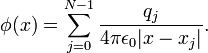
The factor of  in the denominator is annoying to keep around, so we will adopt "computational units". This means that we'll rescale the potential, positions and/or the charges so that, in the new units of measurement,
  . Then the formula for the potential simplifies to
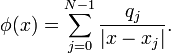
Our goal now is to write a computer program which takes a set of positions and charges as its input, and plots the resulting electric potential.
Writing into a Python source code file
Before writing any Python code, we should create a file to put the code in. On GNU/Linux, fire up your preferred text editor and open an empty file, naming it potentials.py. On Windows, in the window that was opened up by the IDLE (Python GUI) program, click on the menu-bar item File → New File; then type Ctrl-s (or click on File → New File) and save the empty file as potentials.py.
The file extension .py denotes it as a Python source code file. You should save the file in an appropriate directory.
Now let's do a very crude "first pass" at the program. Instead
of handling an arbitrary number of particles, let's assume there's a single particle with some position and charge  . Then we'll plot its potential. Type the following into the file:
from scipy import *
import matplotlib.pyplot as plt

x0 = 1.5
q0 = 1.0

X   = linspace(-5, 5, 500)
phi = q0 / abs(X - x0)

plt.plot(X, phi)
plt.show()
Save the file. Now we will run the program. On GNU/Linux, open a text terminal and cd to the directory where you file is, then type python -i potentials.py. On Windows, while in file-editing window type F5 (or click on Run → Run Module). In either case, you should see a figure pop up:
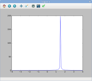
That's pretty much what we expect: the potential is peaked at  , which is the position of the particle we specified in the program (via the variable named
 x0). The charge of the particle is given by the variable named q0, and we have assigned that the value 1.0. Hence, the potential is positive.
Now close the figure, and return to the Python command prompt. Note that Python is still running, even though your program has finished. From the command line, you can also examine the values of the variables which have been created by your program, simply by typing their names into the command prompt:
>>> x0
1.5
>>> phi
array([ 0.15384615    0.15432194    0.15480068    0.1552824  ....
          ....        0.28902404    0.28735963    0.28571429 ])
The value of x0 is a number, 1.5, which was assigned to it when our program ran. The value of phi is more complicated: it is an array,
which is a special data structure containing a sequence of numbers.
From the command line, you can inspect the individual elements of this
array. For example, to see the value of the array's first element, type
this:
>>> phi[0]
0.153846153846
As we've mentioned, index 0 refers to the first element of the array. This so-called zero-based indexing is a common practice in computing. Similarly, index 1 refers to the second element of the array, index 2 refers to the third element, etc.
You can also look at the length of the array, by calling the function len. This function accepts an array input and returns its length, as an integer.
>>> len(phi)
500
You can exit the Python command line at any time by typing Ctrl-d or exit().
Modularizing the code
Designing a potential function
We could continue altering the above code in a straightforward way.
For example, we could add more particles by adding variables x1, x2, q1, q2, and so forth, and altering our formula for computing phi.
However, this is not very satisfactory: each time we want to consider a
new collection of particle positions or charges, or change the number
of particles, we would have to re-write the program's internal
"logic"—i.e., the part that computes the potentials. In programming
terminology, our program is insufficiently "modular". Ideally, we want
to isolate the part of the program that computes the potential from the
part that specifies the numerical inputs to the calculation, like the
positions and charges.
To modularize the code, let's define a function that computes the potential of an arbitrary set of charged particles, sampled at an arbitrary set of positions. Such a function would need three sets of inputs:
- An array of particle positions
![\vec{x} \equiv [x_0, \cdots, x_{N-1}]](PH4505_files/21ff42368bcbe9319c2a6f3b7f9b4856.png) . (Don't get confused, by the way: we are using these numbers to refer to the positions of particles in a 1D space, not the position of a single particle in an -dimensional space.)
. (Don't get confused, by the way: we are using these numbers to refer to the positions of particles in a 1D space, not the position of a single particle in an -dimensional space.)
- An array of particle charges
![\vec{q} \equiv [q_0, \cdots, q_{N-1}]](PH4505_files/5dab4dd8ec74430cf2cc154ffea2e1d8.png) .
.
- An array of sampling points
![\vec{X} \equiv [X_0, \cdots, X_{M-1}]](PH4505_files/a6e123472e19b6123e66c010c8abc95b.png) , which are the points where we want to know
, which are the points where we want to know  .
.
The number of particles, , and the number of sampling points,  , should be arbitrary positive integers. Furthermore, and need not be equal.
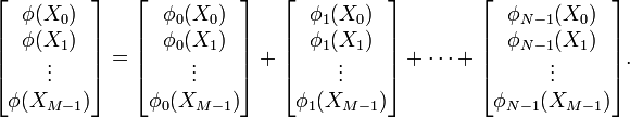
The function we intend to write must compute the array
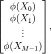
which contains the value of the total electric potential at each of
the sampling points. The total potential can be written as the sum of
contributions from all particles. Let us define  as the potential produced by particle
  :
:
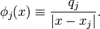
Then the total potential is
Writing the program
Let's code this up. Return to the file potentials.py, and delete the entire contents of the file. Then replace it with the following:
from scipy import *
import matplotlib.pyplot as plt

## Return the potential at measurement points X, due to particles
## at positions xc and charges qc.  xc, qc, and X must be 1D arrays,
## with xc and qc of equal length.  The return value is an array
## of the same length as X, containing the potentials at each X point.
def potential(xc, qc, X):
    M = len(X)
    N = len(xc)
    phi = zeros(M)
    for j in range(N):
        phi += qc[j] / abs(X - xc[j])
    return phi

charges_x  = array([0.2, -0.2])
charges_q  = array([1.5, -0.1])
xplot = linspace(-3, 3, 500)

phi = potential(charges_x, charges_q, xplot)

plt.plot(xplot, phi)
pmin, pmax = -50, 50
plt.ylim(pmin, pmax)
plt.show()
When typing or pasting the above into your file, be sure to preserve the indentation (i.e., the number of spaces at the beginning of each line). Indentation is important in Python; as we'll see, it's used to determine program structure. Now save and run the program again:
- In the Windows GUI, type
F5in the editing window showingpotentials.py. - On GNU/Linux, type
python -i potentials.pyfrom the command line. - Alternatively, from the Python command line, type
import potentials, which will load and run yourpotentials.pyfile.
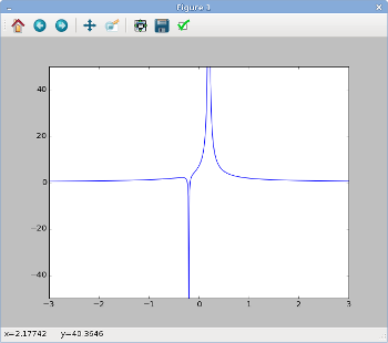
You should now see a figure like the one on the right, showing the
electric potential produced by two particles, one at position  with charge
  and the other at position
  with charge
  .
.
There are less than 20 lines of actual code in the above program, but they do quite a lot of things. Let's go through them in turn:
Module imports
The first two lines import the Scipy and Matplotlib modules, for use in our program. We have not yet explained how importing works, so let's do that now.
from scipy import *
import matplotlib.pyplot as plt
Each Python module, including Scipy and Matplotlib, defines a variety of functions and variables. If you use multiple modules, you might have a situation where, say, two different modules each define a function with the same name, but doing entirely different things. That would be Very Bad. To help avoid this, Python implements a concept called a namespace. Suppose you import a module (say Scipy) like this:
import scipy
One of the functions defined by Scipy is linspace, which we have already seen. This function was defined by the scipy module, and lies inside the scipy namespace. As a result, when you import the Scipy module using the import scipy line, you have to call the linspace function like this:
x = scipy.linspace(-3, 3, 500)
The scipy. in front says that you're referring to the linspace function that was defined in the scipy namespace. (Note: the online documentation for linspace refers to it as numpy.linspace, but the exact same function is also present in the scipy namespace. In fact, all numpy.* functions are replicated in the scipy namespace. So unless stated otherwise, we only have to import scipy.)
We will be using a lot of functions that are defined in the scipy namespace. Since it would be annoying to have to keep typing scipy. all over the place, we opt to use a slightly different import statement:
from scipy import *
This imports all the functions and variables in the scipy namespace directly into your program's namespace. Therefore, you can just call linspace, without the scipy.
prefix. Obviously, you don't want to do this for every module you use,
otherwise you'll end up with the name-clashing problem we alluded to
earlier! The only module we'll use this shortcut with is scipy.
Another way to avoid having to type long prefixes is shown by this line:
import matplotlib.pyplot as plt
This imports the matplotlib.pyplot module (i.e., the pyplot module which is nested inside the matplotlib module). That's where plot, show, and other plotting functions are defined. The as plt in the above line says that we will refer to the matplotlib.pyplot namespace as the short form plt instead. Hence, instead of calling the plot function like this:
matplotlib.pyplot.plot(x, y)
we will call it like this:
plt.plot(x, y)
Comments
Let's return to the program we were looking at earlier. The next few lines, beginning with #, are "comments". Python ignores the # character and everything that follows it, up to the end of the line. Comments are very important, even in simple programs like this.
When you write your own programs, please remember to include comments. You don't need a comment for every line of code—that would be excessive—but at a minimum, each function should have a comment explaining what it does, and what the inputs and return values are.
Function definition
Now we get to the function definition for the function named potential, which is the function that computes the potential:
def potential(xc, qc, X):
    M = len(X)
    N = len(xc)
    phi = zeros(M)
    for j in range(N):
        phi += qc[j] / abs(X - xc[j])
    return phi
The first line, beginning with def, is a function header. This function header states that the function is named potential, and that it has three inputs. In computing terminology, the inputs that a function accepts are called parameters. Here, the parameters are named xc, qc and X. As explained by the comments,
we intend to use these for the positions of the particles, the charges
of the particles, and the positions at which to measure the potential,
respectively.
The function definition consists of the function header, together the rest of the indented lines below it. The function definition terminates once we get to a line which is at the same indentation level as the function header. (That terminating line is considered a separate line of code, which is not part of the function definition).
By convention, you should use 4 spaces per indentation level.
The indented lines below the function header are called the function body. This is the code that is run each time the function is called. In this case, the function body consists of six lines of code, which are intended to compute the total electric potential, according to the procedure that we have outlined in the preceding section:
- The first two lines define two helpful variables,
MandN. Their values are set to the lengths of theXandxcarrays, respectively. - The next line calls the
zerosfunction. The input tozerosisM, the length of theXarray (i.e., our function's third parameter). Therefore,zerosreturns an array, of the same same length asX, with every element set to 0.0. For now, this represents the electric potential in the absence of any charges. We give this array the namephi. - The function then iterates over each of the particles and add
up its contribution to the potential, using a construct known as a
forloop. The codefor j in range(N):is the loop's "header line", and the next line, indented 4 spaces deeper than the header line, is the "body" of the loop.The header line states that we should run the loop body several times, with the variable
jset to different values during each run. The values ofjto loop over are given byrange(N). This is a function call to the range function, withN(the number of electric charges) as the input. Therange(N)function call returns a sequence specifyingNsuccessive integers, from 0 toN-1, inclusive. (Note that the last value in the sequence isN-1, notN. Because we start from 0, this means that there is a total ofNintegers in the sequence. Also, callingrange(N)is the same as callingrange(0,N).) - For each
j, we computeqc[j] / abs(X - xc[j]). This is an array whose elements are the values of the electric potential at the set of positionsX, arising from the individual particle. In mathematical terms, we are calculating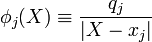
using the array of positions
X. We then add this array tophi. Once this is done for allj, the arrayphiwill contain the desired total potential,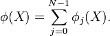
- Finally, we call
returnto specify the function's output, or return value. This is the arrayphi.
Top-level code: numerical constants
After the function definition comes the code to use the function:
charges_x  = array([0.2, -0.2])
charges_q  = array([1.5, -0.1])
xplot = linspace(-3, 3, 500)
Like the import statements at the beginning of the program, these lines of code lie at top level, i.e., they are not indented. The function header which defines the potential function is also at top level. Running a Python program consists of running its top level code, in sequence.
The above lines define variables to store some numerical constants. In the first two lines, charges_x and charges_q variables store the numerical values of the positions and charges we are interested in. These are initialized using the array function. You may be wondering why the array function call has square brackets nested in commas. We'll explain later, in part 2 of the tutorial.
On the third line, the linspace function call returns an array, whose contents are initialized to the 500 numbers between -3 and 3 (inclusive).
Next, we call the potential function, passing charges_x, charges_q and xplot as the inputs:
phi = potential(charges_x, charges_q, xplot)
These inputs provide the values of the function definition's parameters xc, qc, and X
respectively. The return value of the function call is an array
containing the total potential, evaluated at each of the positions
specified in xplot. This return value is stored as the variable named phi.
Plotting
Finally, we create the plot:
plt.plot(xplot, phi)
pmin, pmax = -50, 50
plt.ylim(pmin, pmax)
plt.show()
We have already seen how the plot and show functions work. Here, prior to calling plt.show, we have added two extra lines to make the potential curve is more legible, by adjust the plot's y-axis bounds. The ylim
function accepts two parameters, the lower and upper bounds of the
y-axis. In this case, we set the bounds to -50 and 50 respectively.
There is an xlim function to do the same for the x-axis.
Notice that in the line pmin, pmax = -50, 50, we set two variables (pmin and pmax)
on the same line. This is a little "syntactic sugar" to make the code a
little easier to read. It's equivalent to having two separate lines,
like this:
pmin = -50
pmax = 50
We'll explain how this construct works in the next part of the tutorial.
