Numbers, Arrays, and Scaling
In this article, we will cover the basic concepts of computation, and explain how they relate to writing programs for scientific computing.
Contents[hide] |
A model of computing
A modern computer is a tremendously complex system, with many things to understand at the level of the hardware, the operating system, and the programming software (e.g. Python). It is helpful to consider a simplified computing model, which is basically a "cartoon" representation of a computer that omits the unimportant facts about how it operates, and focuses on the most important aspects of what a computer program does.
The standard paradigm of computing that we use today is the Von Neumann architecture, which divides a computer into three inter-connected units: processor, memory, and input/output devices. We'll use this as the basis of our simplified model, with an emphasis on the processor and memory parts.
A computer's memory is essentially a chunk of space where we can store numbers. For now, we won't concern ourselves with how the contents of memory are organized or formatted. The processor can read one or more numbers from any locations (or addresses) in memory, perform some basic operations on them, and then write the results into any other addresses. We also make three other important assumptions:
- The capacity is effectively infinite; we don't worry about running out.
- The memory is random-access memory (RAM), meaning that the processor can access any addresses in memory, one after another, with the same speed. (In real life, not all types of memory are random-access. Disk drives, for instance, are not, because the scanning head must physically move to different positions in order to read different parts of memory. However, ordinary computer programs can ignore such details, which are left to the operating system to manage.)
- The processor can only do one thing at a time. For example, if you ask it to read two numbers from memory, that takes twice as long as reading a single number from memory. (Again, real computers violate this assumption to some extent; computers now commonly have multiple processors that can performs multiple operations simultaneously. Our present simple model ignores these complications.)
A program is a set of instructions for the processor. For
example, the following line of code is a program (or part of a program)
that tells the processor to add up four numbers that are currently
stored in memory, and save the result to another memory address labelled
x:
x = a + b + c + d
Because the processor can only do one thing at a time, even a simple
line of code like this involves several sequential steps. The processor
can't simultaneously read all four memory addresses (corresponding to a through d); it must read them one at a time. The following figure shows how the processor might carry out the above addition program:
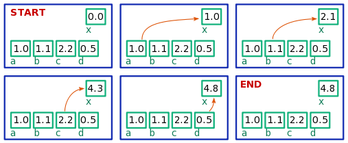
x = a + b + c + d. The computer's memory is visualized as a blue box; the variables x and a through d
correspond to addresses in memory, shown as smaller green boxes
containing numbers. The processor performs the additions one at a time.Integers and floating-point numbers
Digital computers store all data in the form of bits (ones and zeros), and a number is typically stored as a sequence of bits of fixed length. For example, a number labelled x might refer to a sequence of eight bits starting from some specific address, as shown in the following figure:
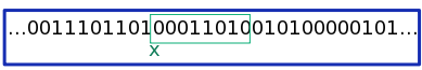
x.The green box indicates the set of memory addresses, eight bits long, where the number is stored. (The other bits, to the left and right of this box, might be used by the computer for other purposes, or simply unused.) What actual number does this sequence of eight bits represent? It depends: there are two types of formats for storing numbers, called integers and floating-point numbers.
Integers
In integer format, one of the bits is used to denote the sign of the
number (positive or negative), and the remaining bits specify an integer
in a binary representation. Because only a fixed number of bits is
available, only a finite range of integers can be represented. On
modern 64-bit computers, integers are typically stored using 64 bits, so
only  distinct integers can be represented. The minimum and maximum integers are


Python is somewhat able to conceal this limitation through a "variable-width integer" feature. If the numbers you're dealing with exceed the above limits, it can convert the numbers to a different format, in which the number of bits can be arbitrarily larger than 64 bits. However, these variable-width integers have various limitations. For one thing, they cannot be stored in a Scipy array meant for storing standard fixed-width integers:
>>> n = array([-2**63])                 # Create an integer array.
>>> n                                   # Check the array's contents.
array([-9223372036854775808])
>>> n.dtype                             # Check the array's data type: it should store 64-bit integers.
dtype('int64')
>>> m = -2**63 - 1                      # If we specify an integer that's too negative, Python makes it variable-width.
>>> m
-9223372036854775809
>>> n[0] = m                            # What if we try to store it in a 64-bit integer array?
Traceback (most recent call last):
  File "<stdin>", line 1, in <module>
OverflowError: Python int too large to convert to C long
Moreover, performing arithmetic operations on variable-width integers is much slower than standard fixed-width arithmetic. Therefore, it's generally best to avoid dealing with integers that are too large or too small.
Floating-point numbers
Floating-point numbers (sometimes called floats) are a format for approximately representing "real numbers"—numbers that are not necessarily integers. Each number is broken up into three components: the "sign", "fraction", and "exponent". For example, the charge of an electron can be represented as

This number can thus be stored as one bit (the sign -), and two integers (the fraction 160217646 and the exponent -27). The two integers are stored in fixed-width format, so the overall floating-point number also has fixed width (64 bits in modern computers). The actual implementation details of floating-point numbers differs from the above example in a few ways—notably, the numbers are represented using powers of 2 rather than powers of 10—but this is the basic idea.
In Python code, floating-point numbers are specified in decimal notation (e.g. 0.000001) or exponential notation (e.g. 1e-6). If you want to represent an integer in floating-point format, give it a trailing decimal point, like this: 3. (or, equivalently, 3.0). If you perform arithmetic between an integer and a floating-point number, like 2 + 3.0, the result is a floating-point number. And if you divide two integers, the result is a floating-point number:
>>> a, b = 6, 3   # a and b are both integers
>>> a/b           # a/b is in floating-point format
2.0
(Note: in Python 2, dividing two integers yielded a rounded integer. This is a frequent source of bugs, so be aware of this behavior if you ever use Python 2.)
Numerical imprecision
Because floating-point numbers use a finite number of bits, the vast majority of real numbers cannot be exactly represented in floating-point format. They can only be approximated. This gives rise to interesting quirks, like this:
>>> 0.1 + 0.1 + 0.1
0.30000000000000004
The reason is that the decimal number 0.1 does not correspond exactly to a floating-point representation, so when you tell the computer to create a number "0.1", it instead approximates that number using a floating-point number whose decimal value is 0.1000000000000000055511512...
Because of this lack of precision, you should not compare floating-point numbers using Python's equality operator ==:
>>> x = 0.1 + 0.1 + 0.1
>>> y = 0.3
>>> x == y
False
Instead of using ==, you can compare x and y by checking if they're closer than a certain amount:
>>> epsilon = 1e-6
>>> abs(x-y) < epsilon
True
The "density" of real numbers represented exactly floating point numbers decreases exponentially with the magnitude of the number. Hence, large floating-point numbers are less precise than small ones. For this reason, numerical algorithms (such as Gaussian elimination) often try to avoid multiplying by very large numbers, or dividing by very small numbers.
Special values
Like integers, floating-point numbers have a maximum and minimum
number that can be represented (this is unavoidable, since they have
only a finite number of bits). Any number above the maximum is assigned
a special value, inf (infinity):
>>> 1e308
1e+308
>>> 1e309
inf
Similarly, any number below the floating-point minimum is represented by -inf. There is another special value called nan (not-a-number), which represents the results of calculations which don't make sense, like "infinity minus infinity":
>>> x = 1e310
>>> x
inf
>>> y = x - x
>>> y
nan
If you ever need to check if a number is inf, you can use Scipy's isinf function. You can check for nan using Scipy's isnan function:
>>> isinf(x)
True
>>> isnan(y)
True
>>> isnan(x)
False
Complex numbers
Complex numbers are not a fundamental data type. Python implements
each complex number as a composite of two floating-point numbers (the
real and imaginary parts). You can spcify a complex number using the
notation X+Yj:
>>> z = 2+1j
>>> z
(2+1j)
Python's arithmetic operations can handle arithmetic operations on complex numbers:
>>> u = 3.4-1.2j
>>> z * u
(8+1j)
>>> z/u
(0.4307692307692308+0.44615384615384623j)
You can retrieve the real and imaginary parts of a complex number using the .real and .imag slots:
>>> z.real
2.0
>>> z.imag
1.0
Alternatively, you can use Scipy's real and imag functions (which also work on arrays). Similarly, the absolute (or abs) and angle functions return the mangnitude and argument of a complex number:
>>> z = 2+1j
>>> real(z)
array(2.0)
>>> imag(z)
array(1.0)
>>> absolute(z)
2.2360679774997898
>>> angle(z)
0.46364760900080609
Arrays
We will often have to deal with collections of several numbers, which requires organizing them into data structures. One of the data structures that we will use most frequently is the array, which is a fixed-size linear sequence of numbers. We have already discussed the basic usage of Scipy arrays in the previous article.
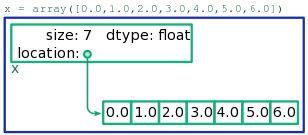
The memory layout of an array is shown schematically in Fig. 3. It consists of two separate regions of memory:
- One region, which we call the book-keeping block, stores summary information about the array, including (i) the total number of elements, (ii) the memory address where the array contents are stored (specifically, the address of element 0), and (iii) the type of numbers stored in the array. The first two pieces of information are recorded in the form of integers, while the last piece is recorded in some other format that we don't need to worry about (it's managed by Python).
- The second region, which we call the data block, stores
the actual contents of the array, laid out sequentially. For example,
for an array containing seven 64-bit integers, this block will consist
of
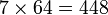 bits of memory, storing the integers one after the other.
The book-keeping block and the data block aren't necessarily kept
next to each other in memory. When a piece of Python code acts upon an
array x, the information in the array's book-keeping block
is used to locate the data block, and then access/alter its data as
necessary.
Basic array operations
Let's take detailed look at what happens when we read or write an individual element of an array, say x[2]: the third element (index 2) stored in the array x.
From the array name, x, Python knows the address of
the relevant book-keeping block (this is handled internally by Python,
and takes negligible time). The book-keeping block records the address
of element 0, i.e. the start of the data block. Because we want index 2
of the array, the processory jumps to the memory address that is 2
blocks past the recorded address. Since the data block is laid out
sequentially, that is precisely the address where the number x[2] is stored. This number can now be read or overwritten, as desired by the Python code.
Under this scheme, the reading/writing of individual array elements is independent of the size of the array. Accessing an element in a size-1 array takes the same time as accessing an element in a size-100000 array. This is because the memory is random-access—the processor can jump to any address in memory once you tell it where to go. The memory layout of an array is designed so that one can always work out the relevant address in a single step.
We describe the speed of this operation using big-O notation. If  is the size of the array, reading/writing individual array elements is said to take
  time, or "order-1 time" (i.e., independent of ). By contrast, a statement like
x.fill(3.3)
takes  time, i.e. time proportional to the array size . That's because the
 fill method assign values to each of the elements of the array. Similarly, the statement
x += 1.0
takes time. This += operation adds 1.0 to each of the elements of the array, which requires arithmetic operations.
Array data type
We have noted that the book-keeping block of each array records the type of number, or data type,
kept in the storage blocks. Thus, each individual array is able to
store only one type of number. When you create an array with the array
function, Scipy infers the data type based on the specified array
contents. For example, if the input contains only integers, an integer
array is created; if you then try to store a floating-point number, it
will be rounded down to an integer:
>>> a = array([1,2,3,4])
>>> a[1] = 3.14159
>>> a
array([1, 3, 3, 4])
In the above situation, if our intention was to create an array of floating point numbers, that can be done by giving the array function an input containing at least one floating-point number. For example,
>>> a = array([1,2,3,4.])
>>> a[1] = 3.14159
>>> a
array([ 1.     ,  3.14159,  3.     ,  4.     ])
Alternatively, the array function accepts a parameter named dtype, which can be used to specify the data type directly:
>>> a = array([1,2,3,4], dtype=float)
>>> a[1] = 3.14159
>>> a
array([ 1.     ,  3.14159,  3.     ,  4.     ])
The dtype parameter accepts several possible values, but most of time you will choose one of these three:
-
float -
complex -
integer
The common functions for creating new arrays, zeros ones, and linspace, create arrays with the float data type by default. They also accept dtype parameters, in case you want a different data type. For example:
>>> a = zeros(4, dtype=complex)
>>> a[1] = 2.5+1j
>>> a
array([ 0.0+0.j,  2.5+1.j,  0.0+0.j,  0.0+0.j])
Vectorization
We have previously discussed the code x += 1.0, which adds 1.0 to every element on the array x. It has runtime , where is the array length. We could also have done the same thing by looping over the array, as follows:
for n in range(len(x)):
    x[n] += 1.0
This, too, has
runtime. But it is not a good way to do the job, for two reasons.
Firstly, it's obviously much more cumbersome to write. Secondly, and
more importantly, it is much more inefficient, because it involves more
"high-level" Python operations. To run this code, Python has to create
an index variable n, increment that index variable times, and increment x[n] for each separate value of n.
By contrast, when you write x += 1.0, Python uses
"low-level" code to increment each element in the array, which does not
require introducing and managing any "high-level" Python objects. The
practice of using array operations, instead of performing explicit loops
over an array, is called vectorization. You should always strive
to vectorize your code; it is generally good programming practice, and
leads to extreme performance gains for large array sizes.
Vectorization does not change the runtime scaling of the operation. The vectorized code x += 1.0, and the explicit loop, both run in time. What changes is the coefficient of the scaling: the runtime has the form 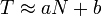 , and the value of the coefficient
  is much smaller for vectorized code.
Here is another example of vectorization. Suppose we have a variable y whose value is a number, and an array x containing a collection of numbers; we want to find the element of x closest to y. Here is non-vectorized code for doing this:
idx, distance = 0, abs(x[0] - y)
for n in range(1, len(x)):
    new_dist = abs(x[n] - y)
    if new_dist < distance:
        idx, distance = n, new_dist

z = x[idx]
The vectorized approach would simply make use of the argmin function:
idx = argmin(abs(x - y))
z = x[idx]
The way this works is to create a new array, whose values are the distances between each element of x and the target number y; then, argmin searches for the array index corresponding to the smallest element (which is also the index of the element of x closest to y). We could write this code even more compactly as
z = x[argmin(abs(x - y))]
Array slicing
We have emphasized that an array is laid out in memory in two pieces: a book-keeping block, and a sequence of storage blocks containing the elements of the array. Sometimes, it is possible for two arrays to share storage blocks. For instance, this happens when you perform array slicing:
>>> x = array([0.0, 1.0, 2.0, 3.0, 4.0, 5.0, 6.0])
>>> y = x[2:5]
>>> y
array([ 2.,  3.,  4.])
The statement y = x[2:5] creates an array named y, containing a subset of the elements of x (i.e., the elements at indices 2, 3, and 4). However, Python does not accomplish this by copying the affected elements of x into a new array with new storage blocks. Instead, it creates a new book-keeping block for y, and points it towards the existing storage blocks of x:
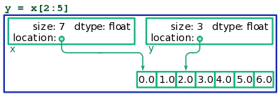
x and y, sharing the same storage blocks.Because the storage blocks are shared between two arrays, if we change an element in x, that effectively changes the contents of y as well:
>>> x[3] = 9.
>>> y
array([ 2.,  9.,  4.])
(The situation is similar if you specify a "step" during slicing, like y = x[2:5:2].
What happens in that case is that the data block keeps track of the
step size, and Python can use this to figure out exactly which address
to jump for accessing any given element.)
The neat thing about this method of sharing storage blocks is that slicing is an
operation, independent of the array size. Python does not need to do
any copying on the stored elements; it merely needs to create a new
book-keeping block. Therefore, slicing is a very "cheap" and efficient
operation.
The downside is that it can lead to strange bugs. For example, this is a common mistake:
>>> x = y = linspace(0, 1, 100)
The above statement creates two arrays, x and y, pointing to the same
storage blocks. This is almost definitely not what we intend! The
correct way is to write two separate array initialization statements.
Whenever you intend to copy an array and change its contents
freely without affecting the original array, you must remember to use
the copy function:
>>> x = array([0.0, 1.0, 2.0, 3.0, 4.0, 5.0, 6.0])
>>> y = copy(x[2:5])
>>> x[3] = 9.
>>> y
array([ 2.,  3.,  4.])
In the above example, the statement y = copy(x[2:5]) explicitly copies out the storage blocks of x. Therefore, when we change the contents of x, the contents of y are unaffected.
Do not call copy too liberally! It is an
operation, so unnecessary copying hurts performance. In particular,
the basic arithmetic operations don't affect the contents of arrays, so
it is always safe to write
>>> y = x + 4
rather than y = copy(x) + 4.
Exercises
- Traditionally, computers keep track of the time/date using a format known as Unix time,
which counts the number of seconds that have elapsed since 00:00:00 UTC
on Thursday, 1 January 1970. But there's a problem if we track Unix
time using a fixed-width integer, since that has a maximum value.
Beyond this date, the Unix time counter will roll-over, wreaking havoc
on computer systems. Calculate the roll-over date for:
- Ordinary (signed) 32-bit integers
- Unsigned 32-bit integers, which do not reserve a bit for the sign (and thus store only non-negative numbers).
- Signed 64-bit integers
- Unsigned 64-bit integers
- Find the runtime of each of the following Python code samples (e.g. or ). Assume that the arrays
xandyare of size:
z = x + yx[5] = x[4]z = conj(x)z = angle(x)x = x[::-1](this reverses the order of elements).
- Write a Python function
uniquify_floats(x, epsilon), which accepts a list (or array) of floatsx, and deletes all "duplicate" elements that are separated from another element by a distance of less thanepsilon. The return value should be a list (or array) of floats that differ from each other by at leasteps. - (Hard) Suppose a floating-point representation uses one sign bit, fraction bits, and
 exponent bits. Find the density of real numbers which can be
represented exactly by a floating-point number. Hence, show that
floating-point precision decreases exponentially with the magnitude of
the number.
exponent bits. Find the density of real numbers which can be
represented exactly by a floating-point number. Hence, show that
floating-point precision decreases exponentially with the magnitude of
the number.
Computational physics notes | Prev: Scipy tutorial (part 2) Next: Numerical linear algebra
