Numerical Integration
In this article, we will look at some basic techniques for numerically computing definite integrals. The most common techniques involve discretizing the integrals, which is conceptually similar to the way we discretized derivatives when studying finite-difference equations.
Contents[hide] |
Mid-point rule
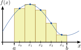
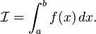
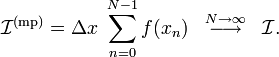
The simplest numerical integration method is called the mid-point rule. Consider a definite 1D integral
Let us divide the range  into a set of
  segments of equal width, as shown in Fig. 1 for the case of
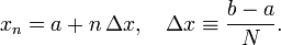
  . The mid-points of these segments are a set of discrete points
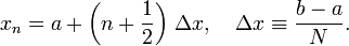
  , where
We then estimate the integral as
The principle behind this formula is very simple to understand. As shown in Fig. 1,  represents the area enclosed by a sequence of rectangles, where the height of each rectangle is equal to the value of
  at its mid-point. As
  ,
the spacing between rectangles goes to zero; hence, the total area
enclosed by the rectangles becomes equal to the area under the curve of .
,
the spacing between rectangles goes to zero; hence, the total area
enclosed by the rectangles becomes equal to the area under the curve of .
Numerical error for the mid-point rule
Let us estimate the numerical error resulting from this
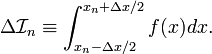
approximation. To do this, consider one of the individual segments,
which is centered at  with length
 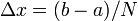 . Let us define the integral over this segment as
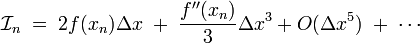
Now, consider the Taylor expansion of in the vicinity of :

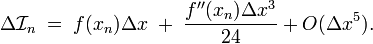
If we integrate both sides of this equation over the segment, the result is
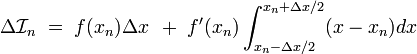

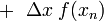
On the right hand side, every other term involves an integrand which is odd around . Such terms integrate to zero. From the remaining terms, we find the following series for the integral of over the segment:
By comparison, the estimation provided by the mid-point rule is simply
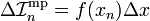
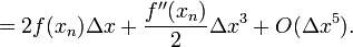
This is simply the first term in the exact series. The remaining terms constitute the numerical error in the mid-point rule integration, over this segment. We denote this error as
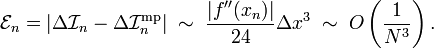
The last step comes about because, by our definition,  .
.
Now, consider the integral over the entire integration range, which consists of
such segments. In general, there is no guarantee that the numerical
errors of each segment will cancel out, so the total error should be times the error from each segment. Hence, for the mid-point rule,
Trapezium rule
The trapezium rule is a simple extension of the mid-point
integration rule. Instead of calculating the area of a sequence of
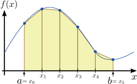
rectangles, we calculate the area of a sequence of trapeziums, as shown
in Fig. 2. As before, we divide the integration region into equal segments; however, we now consider the end-points of these segments, rather than their mid-points. These is a set of  positions
  , such that
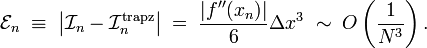
Note that  and
and  . By using the familiar formula for the area of each trapezium, we can approximate the integral as
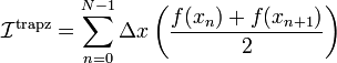
![= \Delta x \left[\left(\frac{f(x_0) + f(x_1)}{2}\right)+ \left(\frac{f(x_1) + f(x_2)}{2}\right) + \cdots + \left(\frac{f(x_{N-1}) + f(x_{N})}{2}\right)\right]](PH4505_files/1b404a7cdc307e67b0661e2e009bba88.png)
![= \Delta x \left[\frac{f(x_0)}{2} + \left(\sum_{n=1}^{N-1} f(x_n)\right) + \frac{f(x_{N})}{2}\right].](PH4505_files/e0b98d015c71ec4a4834f8062450ee1a.png)
Python implementation of the trapezium rule
In Scipy, the trapezium rule is implemented by the trapz function. It usually takes two array arguments, y and x; then the function call trapz(y,x) returns the trapezium rule estimate for  , using the elements of
 x as the discretization points, and the elements of y as the values of the integrand at those points.
Matlab compatibility note: Be careful of the order of inputs! For the Scipy function, it's trapz(y,x). For the Matlab function of the same name, the inputs are supplied in the opposite order, as trapz(x,y).
|
Note that the discretization points in x need not be equally-spaced. Alternatively, you can call the function as trapz(y,dx=s); this performs the numerical integration assuming equally-spaced discretization points, with spacing s.
Here is an example of using trapz to evaluate the integral  :
:
>>> from scipy import *
>>> x = linspace(0,10,25)
>>> y = exp(-x)
>>> t = trapz(y,x)
>>> print(t)
1.01437984777
Numerical error for the trapezium rule
From a visual comparison of Fig. 1 (for the mid-point rule) and Fig. 2
(for the trapezium rule), we might be tempted to conclude that the
trapezium rule should be more accurate. Before jumping to that
conclusion, however, let's do the actual calculation of the numerical
error. This is similar to our above calculation of the mid-point rule's numerical error. For the trapezium rule, however, it's convenient to consider a pair of adjacent segments, which lie between the three discretization points  .
.
As before, we perform a Taylor expansion of in the vicinity of :
If we integrate from  to
to  , the result is

As before, every other term on the right-hand side integrates to zero. We are left with
This has to be compared to the estimate produced by the trapezium rule, which is
![\mathcal{I}_n^{\mathrm{(trapz)}} = \Delta x \left[ \frac{f(x_{n-1})}{2} + f(x_n) + \frac{f(x_{n+1})}{2}\right].](PH4505_files/842ae4ebf59ca95bacd261d90ec33feb.png)
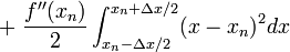
If we Taylor expand the first and last terms of the above expression around , the result is:
![\mathcal{I}_n^{\mathrm{(trapz)}} = \frac{\Delta x}{2} \left[f(x_n) - f'(x_n) \Delta x + \frac{f''(x_n)}{2} \Delta x^2 - \frac{f'''(x_n)}{6} \Delta x^3 + \frac{f''''(x_n)}{24} \Delta x^4 + O(\Delta x^4)\right]](PH4505_files/c7dcebd7c4d6da25a6a7b29b70ea9dbf.png)
![+ \frac{\Delta x}{2} \left[f(x_n) + f'(x_n) \Delta x + \frac{f''(x_n)}{2} \Delta x^2 + \frac{f'''(x_n)}{6} \Delta x^3 + \frac{f''''(x_n)}{24} \Delta x^4 + O(\Delta x^4)\right]](PH4505_files/d530dd4dfe7fe2cb1d1fbdbb0114dd4d.png)
Hence, the numerical error for integrating over this pair of segments is
And the total numerical error goes as
which is the same scaling as the mid-point rule! Despite our expectations, the trapezium rule isn't actually an improvement over the mid-point rule, as far as numerical accuracy is concerned.
Simpson's rule
Our analysis of the mid-point rule and the trapezium rule showed that both methods have  numerical error. In both cases, the error can be traced to the same
source: the fact that the integral estimate over each segment differs
from the Taylor series result in the second-order term—the term proportional to
numerical error. In both cases, the error can be traced to the same
source: the fact that the integral estimate over each segment differs
from the Taylor series result in the second-order term—the term proportional to  .
This suggests a way to improve on the numerical integration result: we
could take a weighted average of the mid-point rule and the trapezium
rule, such that the second-order numerical errors from the two schemes cancel each other out! This is the numerical integration method known as Simpson's rule.
.
This suggests a way to improve on the numerical integration result: we
could take a weighted average of the mid-point rule and the trapezium
rule, such that the second-order numerical errors from the two schemes cancel each other out! This is the numerical integration method known as Simpson's rule.
To be precise, let's again consider a pair of adjacent segments, which lie between the equally-spaced discretization points . As derived above, the integral over these segments can be Taylor expanded as
By comparison, the mid-point rule and trapeium rule estimators for the integral are
Hence, we could take the following weighted average:

Such a weighted average would match the Taylor series result up to  ! (You can check for yourself that the
  terms differ.) In summary, Simpson's rule for this set of three points can be written as
![\mathcal{I}_n^{\mathrm{simp}} = \frac{1}{3} \Big[2f(x_n) \Delta x\Big] + \frac{2}{3} \, \Delta x \Big[ \frac{f(x_{n-1})}{2} + f(x_n) + \frac{f(x_{n+1})}{2}\Big]](PH4505_files/fc760ef5dd833bc854a106cd82737dfb.png)
![= \frac{\Delta x}{3} \Big[f(x_{n-1}) + 4f(x_n) + f(x_{n+1})\Big].](PH4505_files/eb71c22ddedca5cf049d8778c8b5f53c.png)
The total numerical error, over a set of  segments, is
  . That is an improvement of two powers of
  over the trapzezium and mid-point rules! What's even better is that it
involves exactly the same number of arithmetic operations as the
trapezium rule. This is as close to a free lunch as you can get in
computational science.
over the trapzezium and mid-point rules! What's even better is that it
involves exactly the same number of arithmetic operations as the
trapezium rule. This is as close to a free lunch as you can get in
computational science.
Python implementation of Simpson's rule
In Scipy, Simpson's rule is implemented by the scipy.integrate.simps function, which is defined in the scipy.integrate submodule. Similar to the trapz function, this can be called as either simps(y,x) or simps(y,dx=s) to estimate the integral , using the elements of x as the discretization points, with y specifying the set of values for the integrand.
Because Simpson's rule requires dividing the segments into pairs, if you specify an even number of discretization points in x
(i.e. an odd number of segments), the function deals with this by doing
a trapezium rule estimate on the first and last segments. Usually, the
error is negligible, so don't worry about this detail
Here is an example of simps in action:
>>> from scipy import *
>>> from scipy.integrate import simps
>>> x = linspace(0,10,25)
>>> y = exp(-x)
>>> t = simps(y,x)
>>> print(t)
1.00011864276
For the same number of discretization points, the trapezium rule gives  ; the exact result is
  Clearly, Simpson's rule is more accurate.
Gaussian quadratures
Previously, we have assumed in our analysis of numerical integration schemes that the discretization points are equally-spaced. This assumption is not strictly necessary; for instance, we can easily modify the mid-point rule and trapezium rule formulas to work with non-equally-spaced points.
However, if we are free to choose the discretization points for performing numerical integration, and these points need not be equally spaced, then it is possible to exploit this freedom to further improve the accuracy of the numerical integration. The idea is to optimize the placement of the discretization points, so as to minimize the resulting numerical error. This is the basic idea behind the method of integration by Gaussian quadratures.
We will not discuss the details of this numerical integration method. To use it, you can call the scipy.integrate.quad function. This function uses a low-level numerical library named QUADPACK, which performs quadrature integration with adaptive quadratures—i.e.,
it automatically figures out how many discretization points should be
used, and where they should be located, in order to produce a result
with the desired numericaly accuracy.
Because QUADPACK figures out the discretization points for itself, you have to pass quad a function representing the integrand, rather than an array of integrand values as with trapz or simps. The standard way to call the function is
t = quad(f, a, b)
which calculates the integral
The return value is a tuple of the form (t,err), where t is the value of the integral and err is an estimate of the numerical error. The quad
function also accepts many other optional inputs, which can be used to
specify additional inputs for passing to the integrand function, the
error tolerance, the number of subintervals to use, etc. See the documentation for details.
The choice of whether to perform numerical integration using Simpson's rule (simps) or Gaussian quadratures (quad)
is situational. If you already know the values of the integrands at a
pre-determined set of discretization points (e.g., from the result of a finite-difference calculation), then use simps . If you can define a function that can quickly calculate the value of the integrand at any point, use quad.
Here is an example of using quad to compute the integral  :
:
from scipy import *
from scipy.integrate import quad

def f(x):
    return 1.0 / (x*x+1)

integ, _ = quad(f, 0, 1000)
print(integ)
(Note that quad returns two values; the first is the
computed value of the integral, and the other is the absolute error,
which we're not interested in, so we toss it in the "throwaway" variable
named _. See the documentation for details.) Running the above program prints the result  which differs from the exact result,
  by a relative error of
  .
.
Here is another example, where the integrand takes an additional parameter:  :
:
from scipy import *
from scipy.integrate import quad

def f(x, lambd):
    return x * exp(-lambd * x)

integ, _ = quad(f, 0, 100, args=(0.5))
print(integ)
Running the program prints the result  , which agrees with the exact result of
  for the chosen value of the parameter
  .
.
Monte Carlo integration
The final numerical integration scheme that we'll discuss is Monte Carlo integration, and it is conceptually completely different from the previous schemes. Instead of assigning a set of discretization points (either explicitly, as in the mid-point/trapezium/Simpson's rules, or through a machine optimization procedure, as in the adaptive quadrature method), this method randomly samples the points in the integration domain. If the sampling points are independent and there is a sufficiently large number of them, the integral can be estimated by taking a weighted average of the integrand over the sampling points.
To be precise, consider a 1D integral over a domain ![x \in [a,b]](PH4505_files/8290bddba5acf9822dcbf61f4ac67d1b.png) . Let each sampling point be drawn independently from a distribution
. Let each sampling point be drawn independently from a distribution  . This means that the probability of drawing sample in the range
 ![x_n \in [x, x + dx]](PH4505_files/42937aa1629d1df7be7fbcf95a202e86.png) is
is  . The distribution is normalized, so that
Let us take samples, and evaluate the integrand at those points: this gives us a set of numbers  . We then compute the quantity
Unlike the estimators that we have previously studied,  is a random number (because the underlying variables
  are all random). Crucially, its average value is equal to the desired integral:
![= \int_a^b p(x) \, \left[\frac{f(x)}{p(x)}\right]\, dx](PH4505_files/cff780ee8dc976c67fb94e89d23cff0d.png)
For low-dimensional integrals, there is normally no reason to use the Monte Carlo integration method. It requires a much larger number of samples in order to reach a level of numerical accuracy comparable to the other numerical integration methods. (For 1D integrals, Monte Carlo integration typically requires millions of samples, whereas Simpson's rule only requires hundreds or thousands of discretization points.) However, Monte Carlo integration outperforms discretization-based integration schemes when the dimensionality of the integration becomes extremely large. Such integrals occur, for example, in quantum mechanical calculations involving many-body systems, where the dimensionality of the Hilbert space scales exponentially with the number of particles.
Computational physics notes | Prev: Sparse matrix Next: Numerical integration of ODEs
