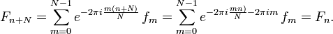
Discrete Fourier Transforms
The Discrete Fourier Transform (DFT) is a discretized version of the Fourier transform, which is widely used in numerical simulation and analysis. Given a set of  numbers
  , the DFT produces another set of numbers numbers
  , defined as follows:

The inverse of this transformation is the Inverse Discrete Fourier Transform (IDFT):

The inverse relationship between the DFT and the IDFT is straightforward to prove, by using the identity
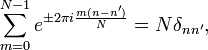
where  denotes the Kronecker delta. This identity is derived from the geometric series formula.
Contents[hide] |
Conversion of continuous Fourier transform to DFT
The DFT is commonly encountered when discretizing formulas involving Fourier integrals. Recall the definition of the Fourier transform: given a function  , where
  , the Fourier transform is a function
  , where
  , and these two functions are related by a pair of integral formulas:
Typically, a computer simulation or experimental measurement will produce values of at certain values of  that are discrete and evenly-spaced. Suppose these points are
  , where the spacing is
  ; the corresponding data points are
  . We are then interested in finding the Fourier spectrum, i.e. plotting either
  or
or  versus
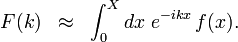
  . To do this, we can approximate the Fourier integral by using the mid-point rule:

Note that this necessitates a truncation of the Fourier integral. The Fourier integral ran over  , but our numerical integral runs over a finite range
  . This truncation will have important consequences later. Now, we have to decide the values of at which to find . Let us choose a set of equally-spaced points,

At these points, the discretized Fourier integral takes the form
![\begin{align}F(k_n) &\approx \Delta x\, \sum_{m=0}^{N-1} \exp\left[- \frac{2 \pi i n (x_0 + m \Delta x)}{N \Delta x}\right] \, f(x_m) \\ &= \Delta x\, \exp\left[- \frac{2 \pi i n x_0}{N \Delta x}\right] \sum_{m=0}^{N-1} e^{-i 2 \pi n m / N} \, f(x_m) \\ &= \Delta x\, \exp\left[- \frac{2 \pi i n x_0}{N \Delta x}\right] \mathrm{DFT}\{f(x_m)\}_n.\end{align}](PH4505_files/168a11ac773fa1237d19d5de63843f1c.png)
Here  denotes the
  -th element of the Discrete Fourier Transform (DFT). The
  index inside the curly brackets is a dummy index, indicating that the
DFT involves an internal sum over this index (we're slightly abusing
mathematical notation here). The phase factor,
index inside the curly brackets is a dummy index, indicating that the
DFT involves an internal sum over this index (we're slightly abusing
mathematical notation here). The phase factor, ![\exp[- 2 \pi i n x_0/N \Delta x]](PH4505_files/ee1ce9087e9edcb70bd29b4f96b94391.png) , is determined by the choice of "origin" for the spatial coordinates; it does not affect
, is determined by the choice of "origin" for the spatial coordinates; it does not affect  (which is what's used to plot the Fourier spectrum).
The DFT and IDFT can be computed very efficiently, in  time, using an algorithm called the Fast Fourier Transform (FFT).
We will not discuss the FFT algorithm in this article, but many good
explanations can be found elsewhere online. In Python, you can perform
an FFT (fast DFT) by calling
time, using an algorithm called the Fast Fourier Transform (FFT).
We will not discuss the FFT algorithm in this article, but many good
explanations can be found elsewhere online. In Python, you can perform
an FFT (fast DFT) by calling fft, and an inverse FFT (fast IDFT) by calling ifft
Spectral resolution and range
In the previous section, we showed how a continuous Fourier integral
is converted into a DFT. This process involved two distinct
approximations. Firstly, the Fourier integral is truncated from its original range, , to a finite interval of length  . Secondly, the integral is discretized by reducing the continuous variable to a set of discrete points
  .
Both of these approximations have important consequences for the
accuracy of our numerical Fourier spectrum, which we will examine in
turn.
.
Both of these approximations have important consequences for the
accuracy of our numerical Fourier spectrum, which we will examine in
turn.
Spectral resolution
 , with
  and sampling interval
 ![k \in [0,300]](PH4505_files/64d39cc86d5ca743b654db7008f11669.png) (about 48 periods).
(about 48 periods).The truncation of the Fourier integral limits the spectral resolution
of the Fourier spectrum. To see this, suppose we perform truncation
without discretization, by taking a continuous Fourier integral and
truncating it to a finite range ![x \in [0, X]](PH4505_files/d74c93c5b906bf1c967813a6ff925541.png) :
:
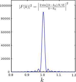
Consider a harmonic function  . The exact Fourier transform can be shown to be a delta function,
  , i.e. an infinitely sharp peak centered at
  . With the above truncation, however, the resulting integral is
![F(k) \;\;\approx\;\; \int_0^X dx \; e^{-i(k - k_0)x} \;\; =\;\; \frac{2\sin[(k-k_0)X/2]}{k-k_0} \cdot e^{-i(k-k_0)X/2}.](PH4505_files/1709af926fb83fdea0f533f22b5d4384.png)
For  , the above formula approaches a delta function (an infinitesimally-thin peak) centered at . But for finite
  , the plot of versus
  behaves as shown in Fig 1. Evidently, truncating the Fourier integral
has "smeared out" the Fourier spectrum, broadening the
infinitesimally-thin delta function peak into a finite-width peak. The
peak width,
behaves as shown in Fig 1. Evidently, truncating the Fourier integral
has "smeared out" the Fourier spectrum, broadening the
infinitesimally-thin delta function peak into a finite-width peak. The
peak width,  , limits the "resolution" of our Fourier analysis.
In the discretized Fourier transform, the truncation of the
Fourier integral has essentially the same effect. As discussed in the previous section, the DFT is defined at  ; hence, the resolution of the Fourier spectrum is
  .
.
Spectral range
The other approximation which we made in going from a continuous Fourier transform to the DFT involved sampling at discrete values of . This discretization has the effect of limiting the spectral range. To see this, let us look again at the DFT formula, which is dimensionless:
Normally, we consider only the indices 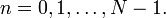 However, if we replace with
  in the right-hand side, the result would be the same:
We can hence regard  as a periodic discrete function of , with period . Next, consider how the DFT is related to the physical and variables. Taking
  for simplicity,
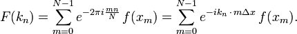
If we perform the replacement
then evidently  is left unchanged. Indeed, we could add any integer multiple of
  without altering the result. This means that the DFT spectrum is only defined under modulo , by contrast with the continuous Fourier transform which is defined over the entire interval
  .
.
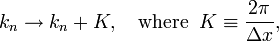
The default definition of the DFT gives the integer indices  , which corresponds to
  . However, when plotting the DFT spectrum, we usually adjust the range of to
  . This is done by taking the "upper half" of the DFT spectrum,
 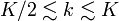 , and translating it via the replacement
  . Due to the periodicity of the DFT, the upper half of the DFT spectrum becomes the negative part of the spectrum. In terms of the integer indices , the process is depicted in the figure below:
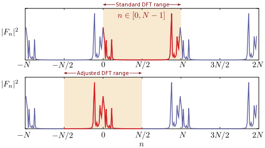
 , is periodic with period . By default, the DFT is reported in the spectral range
 ![n \in [0, N-1]](PH4505_files/bd71e30a8d627a91d7fcdde274ab983b.png) (red curve in the upper plot). To relate this to the continuous Fourier transform, we re-center the spectrum at
(red curve in the upper plot). To relate this to the continuous Fourier transform, we re-center the spectrum at  , which is equivalent to translating the upper half of the spectrum to negative values (red curve in the lower plot).
The reason for this adjustment is that, intuitively, the discretized
Fourier spectrum contains information about the "low-frequency" part of
the spectrum,  , including both positive and negative values of .
On the other hand, the discretized Fourier spectrum lacks information
about the "high frequency" part of the spectrum, which correspond to
harmonics with periods shorter than the discretization step
, including both positive and negative values of .
On the other hand, the discretized Fourier spectrum lacks information
about the "high frequency" part of the spectrum, which correspond to
harmonics with periods shorter than the discretization step  .
Hence, it makes sense to "center" our Fourier spectrum around the
origin. It can then be shown that as the discretization step approaches
zero (and hence
.
Hence, it makes sense to "center" our Fourier spectrum around the
origin. It can then be shown that as the discretization step approaches
zero (and hence  ), the
  part of the adjusted DFT spectrum converges to the exact (continuous) Fourier spectrum.
The corollary to the above discussion is that if we have a function which has no frequency components larger than  , then it is sufficient to use a sampling interval
  . This is called the Nyquist-Shannon sampling theorem.
Summary of spectral relations
The results of the previous sections can be summarized in this way:
- The total range of , which is denoted by , limits the resolution of the spectrum to .
- The resolution of , which is the discretization step , limits the range of the spectrum to
 .
.
These relations are easy to remember, because the "interval length"
in the one domain places a limit on the "discretization step" in the
other domain. It is very important to keep these relations in mind when
working with discrete Fourier transforms! For example, a common
mistake that people make is to try to improve the resolution of a
Fourier spectrum by increasing the number of discretization steps, , while keeping the total interval
fixed. This doesn't work; it leaves the spectral resolution unchanged!
In order to improve the spectral resolution, one has to increase the
total interval instead.
The split-step Fourier method
As an example of the usefulness of the DFT, let us discuss a DFT-based method for performing numerical integration of a partial differential equation, known as the split-step Fourier method. Here, the method will be presented in the context of the time-dependent Schrödinger equation in 1D space:
![i \frac{d\psi(x,t)}{dt} = \left[-\frac{1}{2}\frac{\partial^2}{\partial x^2} + V(x,t)\right]\psi(x,t)](PH4505_files/e92f2a2193422bd714a88108e1d1a50c.png)
We have taken  for simplicity. At each time, the wavefunction is a continuous function of . Let us truncate and discretize this spatial coordinate, by defining a computational domain of length
  containing discretization points:

Thus, the wavefunction at each time is represented by a complex vector, which we call a "state vector":
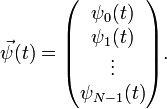
Given an initial state vector  , the problem is to compute
  at a later time
  . Note that this differs from previously-studied numerical ODE problems in one important respect: evolving in time involves taking second-order spatial
derivatives. We won't go into the details, but it turns out that
standard methods for time-stepping and discretizing space don't work
very well here, because the errors from time-stepping and spatial
discretization interact badly with one another. The split-step Fourier
method provides a better way to solve the problem.
. Note that this differs from previously-studied numerical ODE problems in one important respect: evolving in time involves taking second-order spatial
derivatives. We won't go into the details, but it turns out that
standard methods for time-stepping and discretizing space don't work
very well here, because the errors from time-stepping and spatial
discretization interact badly with one another. The split-step Fourier
method provides a better way to solve the problem.
Factorizing the time-evolution operator
The split-step Fourier method is based on the concept of the time-evolution operator. Given a wavefunction  , the wavefunction after a small time step
  is
is
![\psi(x,t_j + \tau) = U(t_j + \tau|t_j)\, \psi(x,t_j), \quad\mathrm{where}\;\;\; U(t_j + \tau|t_j) \approx \exp\left\{-i \tau \left[-\frac{1}{2}\frac{\partial^2}{\partial x^2} + V(x,t_j+\tau/2)\right]\right\}\;.](PH4505_files/36f0a76b4c0c002957d0cac19959efcd.png)
Here, the  refers to the exponential of an operator (one involving spatial derivatives). We call
  the time-evolution operator, which evolves the system from time
  to . The exponential of any operator
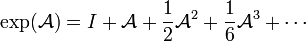
  is defined as the infinite series
In this case, the exponential contains the Hamiltonian, which consists of a kinetic energy term and a potential energy term that do not generally commute. Due to this non-commutivity, the exponential cannot be simplified by factorization:
![\exp\left\{-i \tau \left[-\frac{1}{2}\frac{\partial^2}{\partial x^2} + V(x,t_j+\tau/2)\right]\right\} \;\; \ne\;\;
\exp\Bigg\{\frac{i \tau}{2} \left[\frac{\partial^2}{\partial x^2}\right]\Bigg\} \;
\exp\Bigg\{-i \tau V(x,t_j+\tau/2)\Bigg\}.](PH4505_files/f0bb6d27f8cd9f309c44a1aae720a373.png)
However, we can obtain an approximate factorization by making use of the series definition of the exponential of an operator. One can show that

which is a variant of an important formula known as the Baker–Campbell–Hausdorff formula. On the right-hand side, note that  is sandwiched "symmetrically" between two copies of
  .
This symmetric arrangement reduces the approximation error to third
order, by the cancellation of lower-order errors (in a manner similar to
the mid-point formula for the discretized derivative). Applying this factorization to the time-evolution operator gives
.
This symmetric arrangement reduces the approximation error to third
order, by the cancellation of lower-order errors (in a manner similar to
the mid-point formula for the discretized derivative). Applying this factorization to the time-evolution operator gives
![U(t_j + \tau|t_j) \;\; \approx\;\; U_\mathcal{K} \,\cdot\, U_\mathcal{V}(t_j+\tau/2) \,\cdot\, U_\mathcal{K}, \quad
\mathrm{where}\;\; \begin{cases} \;U_\mathcal{K} &= \exp\left[\frac{i\tau}{4} \frac{d^2}{dx^2}\right] \\ \; U_\mathcal{V}(t) &= \exp\big[-i\tau\, V(x,\,t)\big]\end{cases}](PH4505_files/eafd4232cf8acb066dfbeb47e0b9c2dd.png)
In other words, the time-evolution operator decomposes into three
pieces. That's why we call this a "split-step" algorithm: each time step
from  to
to  consists of applying a kinetic step, then applying a potential step, then applying another kinetic step, in sequence. As previously noted, we'll be working with state vectors (complex -component
vectors), defined through spatial discretization of the wavefunction.
So we need to figure out how the above stepping operators act on these
state vectors:
consists of applying a kinetic step, then applying a potential step, then applying another kinetic step, in sequence. As previously noted, we'll be working with state vectors (complex -component
vectors), defined through spatial discretization of the wavefunction.
So we need to figure out how the above stepping operators act on these
state vectors:
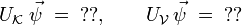
The potential stepping operator is simple to deal with. Since the state vector represents the wavefunction at different points in space, the potential operator is represented by a diagonal matrix, and its exponential is also diagonal:
![U_\mathcal{V} \begin{pmatrix}\psi_0\\ \vdots \\ \psi_{N-1}\end{pmatrix} \;=\; \begin{pmatrix}\exp\left[-i\tau V(x_0,t+\frac{\tau}{2})\right] & & \\ &\ddots&\\ && \exp\left[-i\tau V(x_{N-1},t+\frac{\tau}{2})\right] \end{pmatrix} \begin{pmatrix}\psi_0\\ \vdots \\ \psi_{N-1}\end{pmatrix} \;=\; \begin{pmatrix}\exp\left[-i\tau V(x_0,t+\frac{\tau}{2})\right] \psi_0\\ \vdots \\ \exp\left[-i\tau V(x_{N-1}, t+\frac{\tau}{2})\right]\psi_{N-1}\end{pmatrix}](PH4505_files/f8579ff834b49487674a3b155b7a8299.png)
Kinetic step
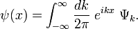
The kinetic stepping operator,  , is less obvious. It contains spatial derivatives and is thus not diagonal in the current basis. The key thing to realize, however, is that this operator is diagonal in wavenumber space. Let us return to the continuous wavefunction, and write its Fourier representation:
Then
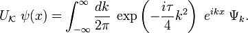
Let us discretize space in steps of , as discussed earlier, and also discretize the Fourier integrals by steps of  :
:
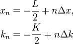
The values of and will be chosen shortly. The discretized integrals become
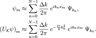
Let us now choose the k-space discretization parameters to be

With this choice, we can show with a bit of algebra that the integral for  reduces to an IDFT:
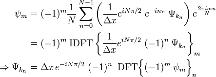
Likewise,
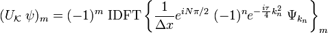
Putting these results together, we get
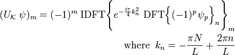
Hence, the  kinetic stepping operator can be implemented by taking a DFT, multiplying the resulting vector elements by
 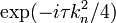 phase factors, and taking an IDFT. The runtime of the stepping process is
 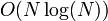 . The , , and
  indices all run over the range
 ![[0, 1, \cdots, N-1]](PH4505_files/4aa58a70b58b45e07567171fecb1547a.png) , consistent with the standard definition of the DFT and IDFT.
, consistent with the standard definition of the DFT and IDFT.
Computational physics notes | Prev: Numerical integration of ODEs Next: Markov chains
