Numerical Integration of ODEs
This article describes the numerical methods for solving the initial-value problem, which is a standard type of problem appearing in many fields of physics. Suppose we have a system whose state at time  is described by a vector
  , which obeys the first-order ordinary differential equation (ODE) for the form:
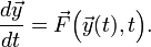
Here,  is some given vector-valued function, whose inputs are (i) the instantaneous state and (ii) the current time . Then, given an initial time
  and an initial state
  , the goal is to find for subsequent times.
Conceptually, the initial value problem is distinct from the problem of solving an ODE discussed in the article on finite-difference equations.
There, we were given a pair of boundaries with certain boundary
conditions, and the goal was to find the solution between the two
boundaries. In this case, we are given the state at an initial time , and our goal is to find for some set of future times  . This is sometimes referred to as "integrating" the ODE, because the solution has the form
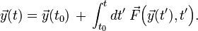
However, unlike ordinary numerical integration (i.e., the computing of a definite integral), the value of the integrand is not known in advance, because of the dependence of on the unknown .
Contents[hide] |
Example: equations of motion in classical mechanics
The above standard formulation of the initial-value problem can be
used to describe a very large class of time-dependent ODEs found in
physics. For example, suppose we have a classical mechanical particle
with position  , subject to an arbitrary external space-and-time-dependent force
  and a friction force
  (where
  is a damping coefficient). Newton's second law gives the following equation of motion:
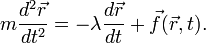
This is a second-order ODE, whereas the standard initial-value problem involves a first-order ODE. However, we can turn it into a first-order ODE with the following trick. Define the velocity vector

and define the state vector by combining the position and velocity vectors:

Then the equation of motion takes the form
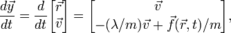
which is a first-order ODE, as desired. The quantity on the right-hand side is the derivative function  for the initial-value problem. Its dependence on and
  is simply regarded as a dependence on the upper and lower portions of the state vector
  . In particular, note that the derivative function does not need to be linear, since
  can have any arbitrary nonlinear dependence on , e.g. it could depend on the quantity
  .
.
The "initial state", ,
requires us to specify both the initial position and velocity of the
particle, which is consistent with the fact that the original equation
of motion was a second-order equation, requiring two sets of initial
values to fully specify a solution. In a similar manner, ODEs of higher
order can be converted into first-order form, by defining the higher
derivatives as state variables and increasing the size of the state
vector.
Forward Euler Method
The Forward Euler Method is the conceptually simplest method for solving the initial-value problem. For simplicity, let us discretize time, with equal spacings:

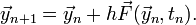
Let us denote  . The Forward Euler Method consists of the approximation
Starting from the initial state  and initial time , we apply this formula repeatedly to compute
  and so forth. The Forward Euler Method is called an explicit method, because, at each step
  , all the information that you need to calculate the state at the next time step,
  , is already explicitly known—i.e., you just need to plug
  and
and  into the right-hand side of the above formula.
The Forward Euler Method formula follows from the usual definition of the derivative, and becomes exactly correct as  . We can deduce the numerical error, which is called the local truncation error in this context, by Taylor expanding the left-hand side around
  :
:
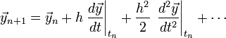
The first two terms are precisely equal to the right-hand side of the
Forward Euler Method formula. The local truncation error is the
magnitude of the remaining terms, and hence it scales as  .
.
Instability
 , for
, for  ,
,  , and
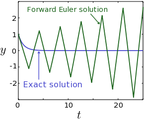
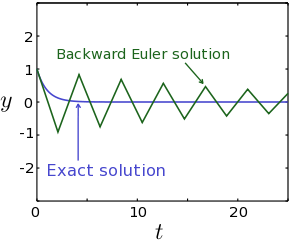
, and  . The numerical solution is unstable; it blows up at large times, even though the exact solution is decaying to zero.
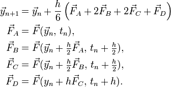
For the Forward Euler Method, the local truncation error leads to a profound problem known as instability. Because the method involves repeatedly applying a formula with a local truncation error at each step, it is possible for the errors on successive steps to progressively accumulate, until the solution itself blows up. To see this, consider the differential equation

Given an initial state  at time
  , the solution is
 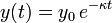 . For
. For  , this decays exponentially to zero with increasing time. However, consider the solutions produced by the Forward Euler Method:
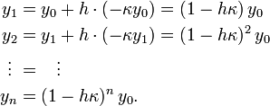
If  , then
 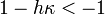 , and as a result
  as
as  .
Even though the actual solution decays exponentially to zero, the
numerical solution blows up, as shown in Fig. 1. Roughly speaking, the
local truncation error causes the numerical solution to "overshoot" the
true solution; if the step size is too large, the magnitude of the
overshoot keeps growing with each step, destabilizing the numerical
solution.
.
Even though the actual solution decays exponentially to zero, the
numerical solution blows up, as shown in Fig. 1. Roughly speaking, the
local truncation error causes the numerical solution to "overshoot" the
true solution; if the step size is too large, the magnitude of the
overshoot keeps growing with each step, destabilizing the numerical
solution.
Stability is a fundamental problem for the integration of ODEs.
The equations which tend to destabilize numerical ODE solvers are those
containing spring constants which are "large" compared to the time step;
such equations are called stiff equations. At first, you might think that it's no big deal: just make the step size  sufficiently small, and the blow-up can be avoided. The trouble is
that it's often unclear how small is sufficiently small, particularly
for complicated (e.g. nonlinear) ODEs, where
sufficiently small, and the blow-up can be avoided. The trouble is
that it's often unclear how small is sufficiently small, particularly
for complicated (e.g. nonlinear) ODEs, where  is something like a "black box". Unlike the above simple example, we
typically don't have the exact answer to compare with, so it can be hard
to tell whether the numerical solution blows up because that's how the
true solution behaves, or because the numerical method is unstable.
is something like a "black box". Unlike the above simple example, we
typically don't have the exact answer to compare with, so it can be hard
to tell whether the numerical solution blows up because that's how the
true solution behaves, or because the numerical method is unstable.
Backward Euler Method
In the Backward Euler Method, we take
Comparing this to the formula for the Forward Euler Method, we see
that the inputs to the derivative function involve the solution at step  , rather than the solution at step . As , both methods clearly reach the same limit. Similar to the Forward Euler Method, the local truncation error is .
Because the quantity appears in both the left- and right-hand sides of the above equation, the Backward Euler Method is said to be an implicit method (as opposed to the Forward Euler Method, which is an explicit method). For general derivative functions  , the solution for cannot be found directly, but has to be obtained iteratively, using a numerical approximation technique such as Newton's method. This makes the Backward Euler Method substantially more complicated to implement, and slower to run.
However, implicit methods like the Backward Euler Method have a
powerful advantage: it turns out that they are generally stable
regardless of step size. By contrast, explicit methods—even explicit
methods that are much more sophisticated than the Forward Euler Method,
like the Runge-Kutta methods
discussed below—are unstable when applied to stiff problems, if the step
size is too large. To illustrate this, let us apply the Backward Euler
Method to the same ODE, , discussed previously. For this particular ODE, the implicit equation can be solved exactly, without having to use an iterative solver:

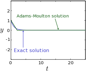
From this result, we can see that the numerical solution does not blow up for large values of , as shown for example in Fig. 2. Even though the numerical solution in this example isn't accurate (because of the large value of ), the key point is that the error does not accumulate and cause a blow-up at large times.
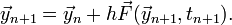
Adams-Moulton Method
In the Second-Order Adams-Moulton (AM2) method, we take
![\vec{y}_{n+1} = \vec{y}_n + \frac{h}{2}\left[ \vec{F}(\vec{y}_{n}, t_{n}) + \vec{F}(\vec{y}_{n+1}, t_{n+1})\right].](PH4505_files/9eabe9589fc323b7e85ed9073029b972.png)
Conceptually, the derivative term here is the average of the Forward Euler and Backward Euler derivative terms. Because
appears on the right-hand side, this is an implicit method. Thus, like
the Backward Euler Method, it typically has to be solved iteratively,
but is numerically stable. The advantage of the AM2 method is that its
local truncation error is substantially lower. To see this, let us take
the derivative of both sides of the ODE over one time step:
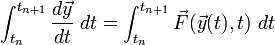
The integral on the left-hand side reduces to  . As for the integral on the right-hand side, if we perform this integral numerically using the trapezium rule, then the result is the derivative term in the AM2 formula. The local truncation error is given by the numerical error of the trapezium rule, which is
  .
That's an improvement of one order compared to the Euler methods.
(Based on this argument, we can also see that the Forward Euler method
and the Backward Euler methods involve approximating the integral on the
right-hand side using a rectangular area, with height given by the
value at and
.
That's an improvement of one order compared to the Euler methods.
(Based on this argument, we can also see that the Forward Euler method
and the Backward Euler methods involve approximating the integral on the
right-hand side using a rectangular area, with height given by the
value at and  respectively. From this, it's clear why the AM2 scheme gives better results.)
There are also higher-order Adams-Moulton methods, which generate
even more accurate results by also sampling the derivative function at
previous steps: 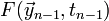 ,
,  , etc.
In Fig. 3, we plot the AM2 solution for the problem , using the same parameters (including the same step size ) as in Fig. 1 (Forward Euler Method) and Fig. 2 (Backward Euler Method). It is clear that the AM2 results are significantly more accurate.
Runge-Kutta methods
The three methods that we have surveyed thus far (Forward Euler,
Backward Euler, and Adams-Moulton) have all involved sampling the
derivative function  at one of the discrete time steps
  , and the solutions at those time steps
  . It is natural to ask whether we can improve the accuracy by sampling the derivative function at "intermediate" values of and . This is the basic idea behind a family of numerical methods known as Runge-Kutta methods.
Here is a simple version of the method, known as second-order Runge-Kutta (RK2). Our goal is to replace the derivative term with a pair of terms, of the form
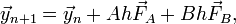
where
The coefficients  are adjustable parameters whose values we'll shortly choose, so as to minimize the local truncation error.
During each time step, we start out knowing the solution at time , we first calculate  (which is the derivative term that goes into the Forward Euler method);
then we use that to calculate an "intermediate" derivative term
(which is the derivative term that goes into the Forward Euler method);
then we use that to calculate an "intermediate" derivative term  . Finally, we use a weighted average of and as the derivative term for calculating . From this, it is evident that this is an explicit method: for each of the sub-equations, the "right-hand sides" contain known quantities.
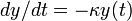
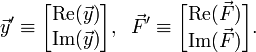
We now have to determine the appropriate values of the parameters . First, we Taylor expand around , using the chain rule:
![\begin{align} \vec{y}_{n+1} &= \vec{y}_n + h \left.\frac{d\vec{y}}{dt}\right|_{t_n} + \frac{h^2}{2} \left.\frac{d^2\vec{y}}{dt^2}\right|_{t_n} + O(h^3)\\
&= \vec{y}_n + h \vec{F}(\vec{y}_n, t_n) + \frac{h^2}{2} \left[ \frac{d}{dt}\vec{F}(\vec{y}(t), t)\right]_{t_n} + O(h^3) \\
&= \vec{y}_n + h \vec{F}(\vec{y}_n, t_n) + \frac{h^2}{2} \left[ \sum_j \frac{\partial \vec{F}}{\partial y_j}\, \frac{dy_j }{dt} + \frac{\partial \vec{F}}{\partial t}\right]_{t_n} + O(h^3) \\
&= \vec{y}_n + h \vec{F}_A + \frac{h^2}{2} \left\{ \sum_j \left[\frac{\partial \vec{F}}{\partial y_j} \right]_{t_n} \!\! F_{Aj} \; +\; \left[\frac{\partial \vec{F}}{\partial t}\right]_{t_n}\right\} + O(h^3) \end{align}](PH4505_files/8a3eec1dfe1e1c63f90da531b605152c.png)
In the same way, we Taylor expand the intermediate derivative term  , whose formula was given above:
![F_B = F_A + \beta \sum_j F_{Aj} \left[\frac{\partial F}{\partial y_j}\right]_{t_n} + \alpha \left[\frac{\partial F}{\partial t}\right]_{t_n}.](PH4505_files/56ca2432e8ed404a51a50b10879a7db1.png)
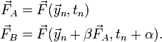
If we compare these Taylor expansions to the RK2 formula, then it can
be seen that the terms can be made to match up to (and including) , if the parameters are chosen to obey the equations
One possible set of solutions is 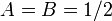 and
and  . With these conditions met, the RK2 method has local truncation error of , one order better than the Forward Euler Method (which is likewise an explicit method), and comparable to the Adams-Moulton Method (which is an implicit method).
The local truncation error can be further reduced by taking more intermediate samples of the derivative function. The most commonly-used Runge-Kutta method is the fourth-order Runge Kutta method (RK4), which is given by
This has local truncation error of  . It is an explicit method, and therefore has the disadvantage of being unstable if the problem is stiff and is sufficiently large.
Integrating ODEs with Scipy
Except for educational purposes, it is almost always a bad idea to implement your own ODE solver; instead, you should use a pre-written solver.
The scipy.integrate.odeint solver
In Scipy, the simplest ODE solver to use is the scipy.integrate.odeint function, which is in the scipy.integrate module. This is actually a wrapper around a low-level numerical library known as LSODE (the Livermore Solver for ODEs"), which is part of a widely-used ODE solver library known as ODEPACK.
The most important feature of this solver is that it is "adaptive": it
can automatically figure out (i) which integration scheme to use
(choosing between either a high-order Adams-Moulton method, or another implicit method known as the Backward Differentiation Formula
which we haven't described), and (ii) the size of the discrete time
steps, based on the behavior of the solutions as they are being worked
out. In other words, the user only needs to specify the derivative
function, the initial state, and the desired output times, without
having to worry about the internal details of the solution method.
The function takes several inputs, of which the most important ones are:
-
func, a function corresponding to the derivative function.
-
y0, either a number or 1D array, corresponding to the initial state.
-
t, an array of times at which to output the ODE solution. The first element corresponding to the initial time. Note that these are the "output" times only—they do not
specify the actual time steps which the solver uses for finding the
solutions; those are automatically determined by the solver.
- (optional)
args, a tuple of extra inputs to pass to the derivative functionfunc. For example, ifargs=(2,3), thenfuncshould accept four inputs, and it will be passed 2 and 3 as the last two inputs.
The function then returns an array y, where y[n] contains the solution at time t[n]. Note that y[0] will be exactly the same as the input y0, the initial state which you specified.
Here is an example of using odeint to solve the damped harmonic oscillator problem 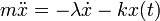 , using the previously-mentioned vectorization trick to cast it into a first-order ODE:
from scipy import *
import matplotlib.pyplot as plt
from scipy.integrate import odeint

def ydot(y, t, m, lambd, k):
    x, v = y[0], y[1]
    return array([v, -(lambd/m) * v - k * x / m])

m, lambd, k = 1.0, 0.1, 1.0   # Oscillator parameters
y0 = array([1.0, 5.0])        # Initial conditions [x, v]
t  = linspace(0.0, 50.0, 100) # Output times

y = odeint(ydot, y0, t, args=(m, lambd, k))

## Plot x versus t
plt.plot(t, y[:,0], 'b-')
plt.xlabel('t')
plt.ylabel('x')
plt.show()
There is an important limitation of odeint: it does not handle complex ODEs, and always assumes that and
are real. However, this is not a problem in practice, because you can
always convert a complex first-order ODE into a real one, by replacing
the complex vectors and with double-length real vectors:
The scipy.integrate.ode solvers
Apart from odeint, Scipy provides a more general interface to a variety of ODE solvers, in the form of the scipy.integrate.ode
class. This is a much more low-level interface; instead of calling a
single function, you have to create an ODE "object", then use the
methods of this object to specify the type of ODE solver to use, the
initial conditions, etc.; then you have to repeatedly call the ODE
object's integrate method, to integrate the solution up to each desired output time step.
The is an extremely aggravating inconsistency between the odeint function and this ode class: the expected order of inputs for the derivative functions are reversed! The odeint function assumes the derivative function has the form F(y,t), but the ode class assumes it has the form F(t,y). Watch out for this!
Here is an example of using ode class with the damped harmonic oscillator problem , using a Runge-Kutta solver:
from scipy import *
import matplotlib.pyplot as plt
from scipy.integrate import ode

## Note the order of inputs (different from odeint)!
def ydot(t, y, m, lambd, k):
    x, v = y[0], y[1]
    return array([v, -(lambd/m) * v - k * x / m])

m, lambd, k = 1.0, 0.1, 1.0   # Oscillator parameters
y0 = array([1.0, 5.0])        # Initial conditions [x, v]
t  = linspace(0.0, 50.0, 100) # Output times

## Set up the ODE object
r = ode(ydot)
r.set_integrator('dopri5')    # A Runge-Kutta solver
r.set_initial_value(y0)
r.set_f_params(m, lambd, k)

## Perform the integration.  Note that the "integrate" method only integrates
## up to one single final time point, rather than an array of times.
x    = zeros(len(t))
x[0] = y0[0]
for n in range(1,len(t)):
    r.integrate(t[n])
    assert r.successful()
    x[n] = (r.y)[0]

## Plot x versus t
plt.plot(t, x, 'b-')
plt.xlabel('t')
plt.ylabel('x')
plt.show()
See the documentation for a more detailed list of options, including the list of ODE solvers that you can choose from.
Computational physics notes | Prev: Numerical integration Next: Discrete Fourier transforms
