Gaussian Elimination
This article discusses the Gaussian elimination algorithm, one of the most fundamental and important numerical algorithms of all time. It is used to solve linear equations of the form

where  is a known
  matrix,
  is a known vector of length
  , and
, and  is an unknown vector of length . The goal is to find . The Gaussian elimination algorithm is implemented by Scipy's
 scipy.linalg.solve function.
There are many good expositions of Gaussian elimination on the web (including the Wikipedia article). Here, we will only go through the basic aspects of the algorithm; you are welcome to read up elsewhere for more details.
Contents[hide] |
The basic algorithm
The best way to understand how Gaussian elimination works is to work through a concrete example. Consider the following  problem:
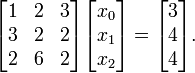
The Gaussian elimination algorithm consists of two distinct phases: row reduction and back-substitution.
Row reduction
In the row reduction phase of the algorithm, we manipulate the matrix equation so that the matrix becomes upper triangular (i.e., all the entries below the diagonal are zero). To achieve this, we note that we can subtract one row from another row, without altering the solution. In fact, we can subtract any multiple of a row.
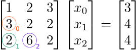
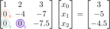
We will eliminate (zero out) the elements below the diagonal in a specific order: from top to bottom along each column, then from left to right for successive columns. For our  example, the elements that we intend to eliminate, and the order in
which we will eliminate them, are indicated by the colored numbers 0, 1,
and 2 in the following figure:
example, the elements that we intend to eliminate, and the order in
which we will eliminate them, are indicated by the colored numbers 0, 1,
and 2 in the following figure:
The first matrix element we want to eliminate is at  (orange circle). To eliminate it, we subtract, from this row, a multiple of row
  . We will use a factor of
  :
:

The factor of  we used is determined as follows: we divide the matrix element at (which is the one we intend to eliminate) by the element at
  (which is the one along the diagonal in the same column). As a result, the term proportional to
  disappears, and we obtain the following modified linear equations, which possess the same solution:
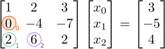
(Note that we have changed the entry in the vector on the right-hand
side as well, not just the matrix on the left-hand side!) Next, we
eliminate the element at  (green circle). To do this, we subtract, from this row, a multiple of row . The factor to use is
  , which is the element at divided by the (diagonal) element:

The result is
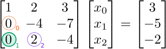
Next, we eliminate the  element (blue circle). This element lies in column
  , so we eliminate it by subtracting a multiple of row . The factor to use is
  , which is the element divided by the
  (diagonal) element:

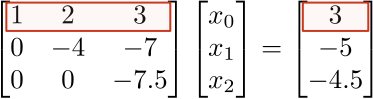
The result is
We have now completed the row reduction phase, since the matrix on the left-hand side is upper-triangular (i.e., all the entries below the diagonal have been set to zero).
Back-substitution
In the back-substitution phase, we read off the solution from the bottom-most row to the top-most row. First, we examine the bottom row:
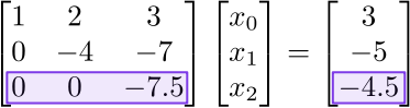
Thanks to row reduction, all the matrix elements on this row are zero except for the last one. Hence, we can read off the solution

Next, we look at the row above:
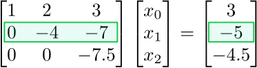
This is an equation involving  and
and  . But from the previous back-substitution step, we know . Hence, we can solve for
![x_1 = [-5 - (-7) (0.6)] / (-4) = 0.2.](PH4505_files/febbaf5b54c3cfa91a54bf78ca8419de.png)
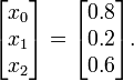
Finally, we look at the row above:
This involves all three variables , , and . But we already know and , so we can read off the solution for . The final result is
Runtime
Let's summarize the components of the Gaussian elimination algorithm, and analyze how many steps each part takes:
| Row reduction | ||||
|---|---|---|---|---|
| • | Step forwards through the rows. For each row  , ,
|
steps
| ||
| • | Perform pivoting (to be discussed below). | 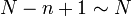 steps steps
| ||
| • | Step forwards through the rows larger than . For each such row  , ,
|
 steps steps
| ||
| • | Subtract  times row from the row (where times row from the row (where  is the current matrix). This eliminates the matrix element at is the current matrix). This eliminates the matrix element at  . .
|
 arithmetic operations arithmetic operations
| ||
| Back-substitution | ||||
| • | Step backwards through the rows. For each row ,
|
steps
| ||
| • | Substitute in the solutions  for for  (which are already found). Hence, find (which are already found). Hence, find  . .
|
 arithmetic operations arithmetic operations
| ||
(The "pivoting" procedure hasn't been discussed yet; we'll do that in a later section.)
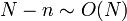
We conclude that the runtime of the row reduction phase scales as  , and the runtime of the back-substitution phase scales as
  . The algorithm's overall runtime therefore scales as .
Matrix generalization
We can generalize the Gaussian elimination algorithm described in the previous section, to solve matrix problems of the form
-
 ,
,
where  and
and  are
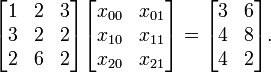
are  matrices, not merely vectors. An example, for
  , is
, is
It can get a bit tedious to keep writing out the  elements in the system of equations, particularly when becomes a matrix. For this reason, we switch to a notation known as the augmented matrix:
![\left[\begin{array}{ccc|cc} 1 & 2 & 3 & 3 & 6 \\ 3 & 2 & 2 & 4 & 8 \\ 2 & 6 & 2 & 4 & 2 \end{array}\right].](PH4505_files/a4ac6e86fb0e0b5e9b63dd3f3c28eb56.png)
Here, the entries to the left of the vertical separator denote the left-hand side of the system of equations, and the entries to the right of the separator denote the right-hand side of the system of equations.
The Gaussian elimination algorithm can now be performed directly on the augmented matrix. We will walk through the steps for the above example. First, row reduction:
- Eliminate the element at :
![\left[\begin{array}{ccc|cc} 1 & 2 & 3 & 3 & 6 \\ 0 & -4 & -7 & -5 & -10 \\ 2 & 6 & 2 & 4 & 2 \end{array}\right]](PH4505_files/e9f45d4ee164df838e2e6595cb18e3e1.png)
- Eliminate the element at :
![\left[\begin{array}{ccc|cc} 1 & 2 & 3 & 3 & 6 \\ 0 & -4 & -7 & -5 & -10 \\ 0 & 2 & -4 & -2 & -10 \end{array}\right]](PH4505_files/df708a22504cc84cea2b950bc381dd9a.png)
- Eliminate the element at :
![\left[\begin{array}{ccc|cc} 1 & 2 & 3 & 3 & 6 \\ 0 & -4 & -7 & -5 & -10 \\ 0 & 0 & -7.5 & -4.5 & -15 \end{array}\right]](PH4505_files/744339111982b0fcafa6e4e68acbb489.png)
The back-substitution step converts the left-hand portion of the augmented matrix to the identity matrix:
- Solve for row
 :
: ![\left[\begin{array}{ccc|cc} 1 & 2 & 3 & 3 & 3 \\ 0 & -4 & -7 & -5 & -10 \\ 0 & 0 & 1 & 0.6 & 2 \end{array}\right]](PH4505_files/92760915a54ea2c6d6604641c6bcb5ca.png)
- Solve for row :
![\left[\begin{array}{ccc|cc} 1 &\; 2 & \;\;\;3 \;\;& 3 & \;3 \\ 0 & \;1 & \;\;\;0\;\; & 0.2 & \;-1 \\ 0 & \;0 & \;\;\;1\;\; & 0.6 & \;2 \end{array}\right]](PH4505_files/afc35d3a6db1adad40e18e850e2ce7c9.png)
- Solve for row :
![\left[\begin{array}{ccc|cc} 1 & \;0 & \;\;\;0\;\; & 0.8 & \;2 \\ 0 & \;1 & \;\;\;0\;\; & 0.2 & \;-1 \\ 0 & \;0 & \;\;\;1\;\; & 0.6 & \;2 \end{array}\right]](PH4505_files/ba596b7b8ce3d40a4c869913a43cb2d2.png)
After the algorithm finishes, the right-hand side of the augmented matrix contains the result for . Analyzing the runtime using the same reasoning as before, we find that the row reduction step scales as 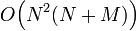 , and the back-substitution step scales as
 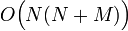 .
.
This matrix form of the Gaussian elimination algorithm is the standard method for computing matrix inverses. If is the identity matrix, then the solution will be the inverse of . Thus, the runtime for calculating a matrix inverse scales as .
Pivoting
In our description of the Gaussian elimination algorithm so far, you
may have noticed a problem. During the row reduction process, we have
to multiply rows by a factor of  (where denotes the current matrix). If
  happens to be zero, the factor blows up, and the algorithm fails.
To bypass this difficulty, we add an extra step to the row reduction procedure. As we step forward through row numbers 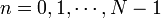 , we do the following for each :
- Pivoting: search through the matrix elements on and below the diagonal element at
 , and find the row
  with the largest value of
  . Then, swap row and row .
- Continue with the rest of the algorithm, eliminating the
 elements below the diagonal.
You should be able to convince yourself that (i) pivoting does not
alter the solution, and (ii) it does not alter the runtime scaling of
the row reduction phase, which remains .
Apart from preventing the algorithm from failing unnecessarily, pivoting improves its numerical stability. If is non-zero but very small in magnitude, dividing by it will produce a very large result, which brings about a loss of floating-point numerical precision. Hence, it is advantageous to swap rows around to ensure that the magnitude of is as large as possible.
When trying to pivot, it might happen that all the values of , on and below the diagonal, are zero (or close enough to zero within our floating-point tolerance). If this happens, it indicates that our original
matrix is singular, i.e., it has no inverse. Hence, the pivoting
procedure has the additional benefit of helping us catch the cases where
there is no valid solution to the system of equations; in such cases,
the Gaussian elimination algorithm should abort.
Example
Let's work through an example of Gaussian elimination with pivoting, using the problem in the previous section:
The row reduction phase goes as follows:
- (
 ): Pivot, swapping row and row :
 ![\left[\begin{array}{ccc|cc} 3 & 2 & 2 & 4 & 8 \\ 1 & 2 & 3 & 3 & 6 \\ 2 & 6 & 2 & 4 & 2 \end{array}\right].](PH4505_files/2c9437d6d368e43244db63fb39dd7e58.png)
- (): Eliminate the element at :
![\left[\begin{array}{ccc|cc} 3 & 2 & 2 & 4 & 8 \\ 0 & 4/3 & 7/3 & 5/3 & 10/3 \\ 2 & 6 & 2 & 4 & 2 \end{array}\right].](PH4505_files/02eabb3262ec825c8821cb15127a8176.png)
- (): Eliminate the element at :
![\left[\begin{array}{ccc|cc} 3 & 2 & 2 & 4 & 8 \\ 0 & 4/3 & 7/3 & 5/3 & 10/3 \\ 0 & 14/3 & 2/3 & 4/3 & -10/3 \end{array}\right].](PH4505_files/8974377eeccd579bc58749798efa9b23.png)
- (
 ): Pivot, swapping row and row :
 ![\left[\begin{array}{ccc|cc} 3 & 2 & 2 & 4 & 8 \\ 0 & 14/3 & 2/3 & 4/3 & -10/3 \\0 & 4/3 & 7/3 & 5/3 & 10/3 \end{array}\right].](PH4505_files/329cbb8ae159f1dc7f1221e442ddf658.png)
- (): Eliminate the element at :
![\left[\begin{array}{ccc|cc} 3 & 2 & 2 & 4 & 8 \\ 0 & 14/3 & 2/3 & 4/3 & -10/3 \\0 & 0 & 15/7 & 9/7 & 30/7 \end{array}\right].](PH4505_files/4c44f5d631f7ce0eacbb0845602b35b5.png)
The back-substitution phase then proceeds as usual. You can check that it gives the same results we obtained before.
LU decomposition
A variant of the Gaussian elimination algorithm can be used to compute the LU decomposition of a matrix. This procedure was invented by Alan Turing, the British mathematician considered the "father of computer science". The LU decomposition of a square matrix consists of a lower-triangular matrix  and an upper-triangular matrix
  , such that

In certain special circumstances, LU decompositions provide a very
efficient method for solving linear equations. Suppose that we have to
solve a set of linear equations  many times, using the same but an indefinite number of 's which might not be known in advance. For example, the 's might represent an endless series of measurement outcomes, with representing some fixed experimental configuration. We would like to efficiently calculate for each that arrives. If this is done with Gaussian elimination, each calculation would take time.
However, if we can perform an LU decomposition ahead of time, then the calculations can be performed much more quickly. The linear equations are

This can be broken up into two separate equations:
Because is lower-triangular, we can solve the first equation by forward-substitution (similar to back-substitution, except that it goes from the first row to last) to find  . Then we can solve the second equation by back-substitution, to find . The whole process takes time, which is a tremendous improvement over performing a wholesale Gaussian elimination.
However, finding the LU decomposition takes time (we won't go into details here, but it's basically a variant of the row reduction phase of the Gaussian elimination algorithm).
Therefore, if we are interested in solving the linear equations only
once, or a handful of times, the LU decomposition method does not
improve performance. It's useful in situations where the LU
decomposition is performed ahead of time. You can think of the LU
decomposition as a way of re-arranging the Gaussian elimination
algorithm, so that we don't need to know during in the first, expensive phase.
In Python, you can perform the LU decomposition using the scipy.linalg.lu function. The forward-substitution and back-substitution steps can be performed using scipy.linalg.solve_triangular.
Computational physics notes | Prev: Numerical linear algebra Next: Eigenvalue problems
