The Markov Chain Monte Carlo Method
The Markov Chain Monte Carlo (MCMC) method is a powerful computational technique based on Markov chains, which has numerous applications in physics as well as computer science.
Contents[hide] |
Basic formulation
The basic idea behind the MCMC method is simple. Suppose we have a set of states labelled by an integer index  , where each state is associated with a probability
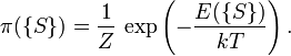
  . For example, in statistical mechanics, for a system maintained at a constant temperature
  , each state occurs with probability
where  is the energy of the state,
  is Boltzmann's constant, and
  is the partition function
From  ,
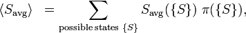
we would like to calculate various expectation values, which describe
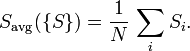
the thermodynamic properties of the system. For example, we might be
interested in the average energy, which is defined as
,
we would like to calculate various expectation values, which describe
the thermodynamic properties of the system. For example, we might be
interested in the average energy, which is defined as
The most straightforward way to find  is to explicitly calculate the above sum. But if the number of states
is very large, this is prohibitively time-consuming (unless there is a
tractable analytic solution, and frequently there isn't). For example,
if we are interested in describing 1000 distinct atoms each having 2
possible energy levels, the total number of states is
is to explicitly calculate the above sum. But if the number of states
is very large, this is prohibitively time-consuming (unless there is a
tractable analytic solution, and frequently there isn't). For example,
if we are interested in describing 1000 distinct atoms each having 2
possible energy levels, the total number of states is  . Trying to calculate a sum over this mind-boggingly many terms would take longer than the age of the universe.
The MCMC method gets around this problem by selectively sampling the states. To accomplish this, we design a Markov process whose stationary distribution is identically equal to the given probabilities . We will discuss how to design the Markov process in the next section. Once we have an appropriate Markov process, we can use it to generate a long Markov chain, and use that chain to calculate moving averages of our desired quantities, like . If the Markov chain is sufficiently long, the average calculated this way will converge to the true expectation value .
The key fact which makes all this work is that the required length of the Markov chain is usually much less than the total number of possible states. For the above-mentioned problem of 1000 distinct two-level atoms, there are  states, but a Markov chain of as few as
  steps can get within several percent of the true value of .
(The actual accuracy will vary from system to system.) The reason for
this is that the vast majority of states are extremely unlikely, and
their contributions to the sum leading to are very small. A Markov chain can get a good estimate for by sampling the states that have the highest probabilities, without spending much time on low-probability states.
steps can get within several percent of the true value of .
(The actual accuracy will vary from system to system.) The reason for
this is that the vast majority of states are extremely unlikely, and
their contributions to the sum leading to are very small. A Markov chain can get a good estimate for by sampling the states that have the highest probabilities, without spending much time on low-probability states.
The Metropolis algorithm
The MCMC method requires us to design a Markov process to match a given stationary distribution .
This is an open-ended problem, and generally there are many good ways
to accomplish this goal. The most common method, called the Metropolis algorithm, is based on the principle of detailed balance, which we discussed in the article on Markov chains.
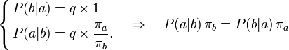
To recap, the principle of detailed balance states that under generic
circumstances (which are frequently met in physics), a Markov process's
transition probabilities are related to the stationary distribution by

The Metropolis algorithm specifies the following Markov process:
- Suppose that on step , the system is in state
 . Randomly choose a candidate state,
  ,
by making an unbiased random step through the space of possible states.
(Just how this choice is made is system-dependent, and we'll discuss
this below.)
,
by making an unbiased random step through the space of possible states.
(Just how this choice is made is system-dependent, and we'll discuss
this below.) - Compare the probabilities and
 :
:
- If
 , accept the candidate.
 - If
 , accept the candidate with probability
  . Otherwise, reject the candidate.
- If
- If the candidate is accepted, the state on step
 is . Otherwise, the state on step remains .
 - Repeat.
Based on the above description, let us verify that the stationary
distribution of the Markov process satisfies the desired
detailed-balance condition. Consider any two states  , and assume without loss of generality that
  . If we start from
  , suppose we choose a candidate step
  with some probability
  . Then, according to the Metropolis rules, the probability of actually making this transition, , is times the acceptance probability
  . On the other hand, suppose we start from
  instead. Because the candidate choice is unbiased, we will choose a candidate step
  with the same probability as in the previous case. Hence, the transition probability for is times the acceptance probability of
  . As a result,
Since this reasoning holds for arbitrary ,
the principle of detailed balance implies that the stationary
distribution of our Markov process follows the desired distribution .
Expression in terms of energies
In physics, the MCMC method is commonly applied to thermodynamic states, for which
In such cases, the Metropolis algorithm can be equivalently expressed in terms of the state energies:
- Suppose that on step , the system is in state . Randomly choose a candidate state, , by making an unbiased random step through the space of possible states.
- Compare the energies and
 :
:
- If
 , accept the candidate.
 - If
 , accept the candidate with probability
 ![\exp\left[(E_n - E_m)/kT\right]](PH4505_files/55ccc4f0859b79903807bc34a993485a.png) . Otherwise, reject the candidate.
. Otherwise, reject the candidate.
- If
- If the candidate is accepted, the state on step is . Otherwise, the state on step remains .
- Repeat.
Stepping through state space
One way of thinking about the Metropolis algorithm is that it takes a scheme for performing an unbiased random walk through the space of possible states (represented by our candidate choices), and converts it into a scheme for performing a biased random walk. The biased random walk corresponds to a Markov process with the stationary distribution we are interested in.
The way the Metropolis candidates are chosen (i.e., the "unbiased
random walk" part) varies from system to system, and once again there
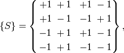
are multiple valid schemes that we could employ. For example, suppose
we have a collection of 6 atoms, where each atom can be in the level
labelled  or the level labelled . Each state of the overall system is described by a list of 6 symbols, e.g.
  .
Then we can make an unbiased walk through the "state space" by
randomly choosing one of the 6 atoms (with equal probability), and
flipping it. For example, we might choose to flip the second atom:
.
Then we can make an unbiased walk through the "state space" by
randomly choosing one of the 6 atoms (with equal probability), and
flipping it. For example, we might choose to flip the second atom:

If we start from the other state, the reverse process has the same probability:

Hence, this scheme for walking through the "state space" is said to be unbiased.
Note that, for a given walking scheme, it is not always possible to
connect every two states by a single step; for example, in this case we
can't go from  to
to  in one step.
There is more than one possible walking scheme; for instance, a different scheme could involve randomly choosing two atoms and flipping them. Whatever scheme we choose, however, the most important thing is that the walk must be unbiased: each possible step must occur with the same probability as the reverse step. Otherwise, the above proof that the Metropolis algorithm satisfies detailed balance would not work.
The Ising model
Problem statement
To better understand the above general formulation of the MCMC method, let us apply it to the 2D Ising model,
a simple and instructive model which is commonly used to teach
statistical mechanics concepts. The system is described by a set of N
"spins", arranged in a 2D square lattice, where the value of each spin  is either
  (spin up) or
  (spin down). This describes a hypothetical two-dimensional magnetic
material, where the magnetization of each atom is constrained to point
either up or down.
(spin down). This describes a hypothetical two-dimensional magnetic
material, where the magnetization of each atom is constrained to point
either up or down.
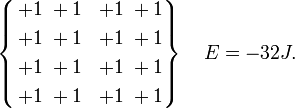
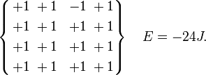
Each state can be described by a grid of  values. For example, for a
  grid, a typical state can be represented as
and the total number of possible states is  .
.
The energy of each state is given by
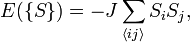
where  denotes pairs of spins, on adjacent sites labelled
  and
and  ,
which are adjacent to each other on the grid (without double-counting).
We'll assume periodic boundary conditions at the edges of the lattice.
Thus, for example,
,
which are adjacent to each other on the grid (without double-counting).
We'll assume periodic boundary conditions at the edges of the lattice.
Thus, for example,
For each state, we can compute various quantities of interest, such as the mean spin
Here,  denotes the average over the lattice, for a given spin configuration. We are then interested in the thermodynamic average
  , which is obtained by averaging
  over a thermodynamic ensemble of spin configurations:
where  denotes the probability of a spin configuration:
Metropolis Monte Carlo simulation
To apply the MCMC method, we design a Markov process using the Metropolis algorithm discussed above. In the context of the Ising model, the steps are as follows:
- On step , randomly choose one of the spins, , and consider a candidate move which consists of flipping that spin:
 .
. - Calculate the change in energy that would result from flipping spin , relative to
 , i.e. the quantity:
![Q \equiv \frac{\Delta E}{kT} = - \left[\frac{J}{kT} \sum_{j\;\mathrm{next}\;\mathrm{to}\;i} S_j\right] \Delta S_i,](PH4505_files/18ccadfa982e7d716adf334d01633e9d.png)
where is the change in
  due to the spin-flip, which is
  if
if  currently, and
  if
if  currently. (The reason we calculate
 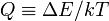 , rather than
  ,
is to keep the quantities in our program dimensionless, and to avoid
dealing with very large or very small floating-point numbers. Note also
that we can do this calculation without summing over the entire
lattice; we only need to find the values of the spins adjacent to the
spin we are considering flipping.)
,
is to keep the quantities in our program dimensionless, and to avoid
dealing with very large or very small floating-point numbers. Note also
that we can do this calculation without summing over the entire
lattice; we only need to find the values of the spins adjacent to the
spin we are considering flipping.)
- If
 , accept the spin-flip.
 - If
 , accept the spin-flip with probability
  . Otherwise, reject the flip.
- If
- This tells us the state on step of the Markov chain (whether the spin was flipped, or remained as it was). Use this to update our moving average of (or whatever other average we're interested in).
- Repeat.
The MCMC method consists of repeatedly applying the above Markov
process, starting from some initial state. We can choose either a
"perfectly ordered" initial state, where  for all spins, or a "perfectly disordered" state, where each is assigned either or randomly.
In some systems, the choice of initial state is relatively
unimportant; you can choose whatever you want, and leave it to the
Markov chain to reach the stationary distribution. For the Ising model,
however, there is a practical reason to prefer a "perfectly ordered"
initial state, for the following reason. Depending on the value of  ,
the Ising model either settles into a "ferromagnetic" phase where the
spins are mostly aligned, or a "paramagnetic" phase where the spins are
mostly random. If the model is in the paramagnetic phase and you start
with an ordered (ferromagnetic) initial state, it is easy for the spin
lattice to "melt" into disordered states by flipping individual spins,
as shown in Fig. 1:
,
the Ising model either settles into a "ferromagnetic" phase where the
spins are mostly aligned, or a "paramagnetic" phase where the spins are
mostly random. If the model is in the paramagnetic phase and you start
with an ordered (ferromagnetic) initial state, it is easy for the spin
lattice to "melt" into disordered states by flipping individual spins,
as shown in Fig. 1:
 lattice with
  . The ordered spin lattice "melts" into a disordered configuration, which is the thermodynamic equilibrium for this value of .
In the ferromagnetic phase, however, if you start with a disordered
initial state, the spin lattice will "freeze" by aligning adjacent
spins. When this happens, large domains with opposite spins will form,
as shown in Fig. 2. These separate domains cannot
be easily aligned by flipping individual spins, and as a result the
Markov chain gets "trapped" in this part of the state space for a long
time, failing to access the more energetically favorable set of states
where most of the spins form a single aligned domain. (The simulation
will eventually get unstuck, but only if you wait a very long time.) The presence of domains will bias the calculation of ,
because the spins in different domains will cancel out. Hence, in this
situation is better to start the MCMC simulation in an ordered state.
lattice with  . As the disordered spin lattice "freezes", it forms long-lasting domains which can interfere with calculations of .